
Past exam of the mathematics course of the University of Cambridge 2006 ia Paper 3 11A Solution Created 2026-09-24 Updated 2026-10-14
Let . It is a harmonic function in the bounded region and vanishes on its entire boundary. For smooth solutions and boundary, the divergence theorem applied to gives the energy identityThe integrand is nonnegative, so in . Thus is constant on each connected component, and its zero Dirichlet boundary condition makes every constant zero. HenceThis proves the Uniqueness of the Dirichlet problem rather than assuming it.
For the separated expression, write . The hyperbolic factor obeys and the trigonometric factor obeys , sofor all the constants, including . In the half-strip take so the region has positive width. For every nonzero integer , the decaying harmonic sine mode in a half-strip isIts second derivatives cancel, it vanishes at , and it has the prescribed sine trace at . The absolute value in the exponential ensures decay for negative as well as positive . For , the zero function is the solution. Thus all integer cases are covered, and the decay is uniform across the strip.
Past exam of the mathematics course of the University of Cambridge 2006 ia Paper 3 10A Solution Created 2026-09-24 Updated 2026-10-14
For a smooth vector field near an oriented piecewise smooth surface , Stokes theorem stateswhere the boundary orientation is induced by the surface unit normal through the right-hand rule. For a constant vector , the curl of is . Apply Stokes theorem and use the scalar triple product:Since this holds for every constant , equality of all vector components proves the vector-valued Stokes identityFor the specified field, the two axis segments contribute zero because vanishes on them. On the arc the direct line integral isIts two terms giveandThereforeOne can also check the orientation and sign by Stokes theorem. For the upward-oriented quarter disk, . Polar integration givesconsistent with the positively oriented boundary in the question.
Past exam of the mathematics course of the University of Cambridge 2006 ia Paper 2 9F Solution Created 2026-09-24 Updated 2026-10-14
Condition on the current generation size. By independence of offspring families, . Taking the expected value gives the probability generating function recursionInduction therefore proves the branching-process generating-function iterationwhere the right side means -fold composition, not an ordinary power.
Let and be the offspring mean and variance, assuming a finite second moment. Differentiating the generating-function recursion at one gives and, with ,Since , this impliesIteration and summation of the geometric progression give the mean and variance of a Galton-Watson generation:For the offspring count is identically zero, so every later generation has zero variance. The zeroth generation always has zero variance. Finiteness of the needed moments is an assumption for this finite-valued variance formula, not a consequence of merely having a probability generating function. With finite positive mean but infinite offspring variance, all positive-generation variances are infinite.
For the total count, make the generation convention explicit. If the first generations include the ancestor, put and , with . Given children of the ancestor, each starts an independent depth- descendant tree with generating function . The ancestor contributes an additional factor , soThis is the finite-horizon total progeny generating function. If instead “first generations” means descendants , excluding , write for that convention. Conditioning on the children now gives , with and . The two conventions encode the same tree but different counts.
Past exam of the mathematics course of the University of Cambridge 2006 ia Paper 2 8B Solution Created 2026-09-24 Updated 2026-10-14
Seek a power series . The initial values give and . Matching the coefficient of for gives . Induction yields , henceThe ratio of successive absolute terms is , so the series and its derivatives converge on every compact interval and satisfy the equation and initial values.
The first recursive approximations are , and . The general formula isIt holds for . Assuming it for , twice integrating with the required initial values gives the Volterra integral equation iterationEach monomial integrates by , producing precisely the next truncated series and proving the induction. The integrand is continuous at zero by its limiting value, since each previous iterate has zero constant term. Thus the Volterra iteration for a singular power-series problem produces successive partial sums, converging with derivatives on compact sets to the analytic solution already found.
Past exam of the mathematics course of the University of Cambridge 2006 ia Paper 2 7B Solution Created 2026-09-24 Updated 2026-10-14
The Wronskian satisfies Abel identity. Differentiating and substituting the homogeneous equations givesso . The two homogeneous solutions are therefore independent.
Define the variation of parameters kernelFor fixed , it satisfies the homogeneous differential equation in . Direct evaluation gives and . For , differentiation under the integral therefore yieldsCombining these identities proves ; both initial values vanish. Continuity of the coefficients gives uniqueness of this initial value problem, establishing the proposed formula rather than merely recognizing it as a standard method.
For the oscillator, , and , so the kernel is . HenceUsing and givesThe factor reflects resonance with the homogeneous oscillator frequency.
Past exam of the mathematics course of the University of Cambridge 2006 ia Paper 2 6B iii Created 2026-09-24 Updated 2026-09-24
Past exam of the mathematics course of the University of Cambridge 2006 ia Paper 2 6B ii Created 2026-09-24 Updated 2026-09-24
Past exam of the mathematics course of the University of Cambridge 2006 ia Paper 2 6B i Created 2026-09-24 Updated 2026-09-24
Past exam of the mathematics course of the University of Cambridge 2006 ia Paper 2 5B Solution Created 2026-09-24 Updated 2026-10-14
First solve the closed linear system of differential equations for . Its coefficient matrix is , with characteristic polynomial . Corresponding eigenvectors are and . The homogeneous solution is thereforeUse separate exponential particular solutions for the two forcing frequencies. Solving and gives and . HenceThe third equation then gives . Integrating,The three arbitrary constants span the general solution: two arise from the first-order subsystem and one from integrating .
Past exam of the mathematics course of the University of Cambridge 2006 ia Paper 2 4F Solution Created 2026-09-24 Updated 2026-10-14
Writing , the ordinary probability generating function isIts finite sum can be differentiated termwise, givingThe Dirichlet probability generating function is the different transform . Evaluating at gives the first ordinary moment, whereas differentiation gives . ThereforeThere is no convergence issue because the support is finite and all its values are positive.
Past exam of the mathematics course of the University of Cambridge 2006 ia Paper 2 3F Solution Created 2026-09-24 Updated 2026-10-14
A real function on an interval is a convex function iffor all in its domain and . For a finite-valued random variable with values and probabilities , Jensen's inequality statesApply this with equal probabilities to and the convex function on the nonnegative axis:Multiplying by proves the sharp two-term convex power bound. Conversely taking forces . ThusFor the inequality is equality for every pair; for equality occurs when .
Past exam of the mathematics course of the University of Cambridge 2006 ia Paper 2 2B Solution Created 2026-09-24 Updated 2026-10-14
Substituting an exponential particular solution gives , or . Since is not an eigenvalue of , the matrix is invertible. The exponential forcing of a constant-coefficient differential system therefore hasFor the specified matrix, . Solving , gives , soDifferentiation verifies both component equations directly. If a general solution were desired, the homogeneous term would be added, with the matrix exponential here equal to because .
Past exam of the mathematics course of the University of Cambridge 2006 ia Paper 2 1B Solution Created 2026-09-24 Updated 2026-10-14
The logistic equation has the constant solutions and . For a nonconstant solution, separation of variables givesSolving and imposing the initial value yieldsThis expression also includes the two equilibria when or . For other initial values it is taken on the maximal interval containing on which its denominator does not vanish.
The phase portrait follows from the sign of : arrows point left for , right for , and left for . Thus zero is an unstable equilibrium point and one is asymptotically stable. The requested sketch is shown below.
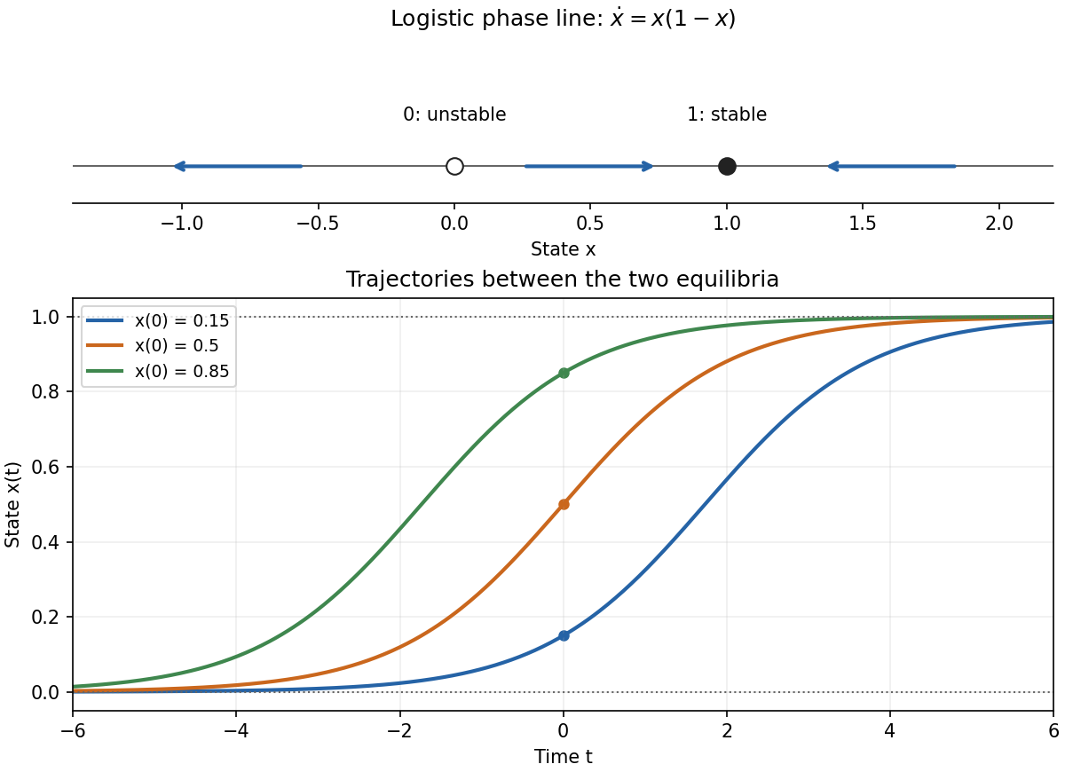
Logistic phase portrait and representative trajectories between the equilibria
. Details. 
If , the denominator is positive for every real . The solution stays between the equilibria and increases monotonically, withMore precisely in the remote past and in the remote future. Outside that interval there is a finite-time pole: for it occurs in the future, and for in the past, at . This does not affect the globally defined trajectories requested between zero and one.
Past exam of the mathematics course of the University of Cambridge 2006 ia Paper 2 12F Solution Created 2026-09-24 Updated 2026-10-14
Normalization uses , henceEach variable therefore has the standard Cauchy distribution. Let . We prove by induction that its probability density function isIt holds for . If it holds for , independence and convolution of probability densities giveThe supplied integral identity makes this , completing the induction. Thus addition increases the Cauchy scale to .
For , the density transformation is , givingThe Cauchy sample mean has an unchanged distribution. In particular, for every ,independently of , so the average does not converge in probability to zero.
There is no contradiction with the usual weak law of large numbers, whose finite-first-moment hypothesis is absent: . The positive and negative parts of both have infinite expectations, so is undefined. Its symmetric principal value is zero, but a principal value is not an expected value. The law therefore supplies no conclusion that these sample averages must approach zero.
Past exam of the mathematics course of the University of Cambridge 2006 ia Paper 2 11F Solution Created 2026-09-24 Updated 2026-10-14
After the top card is fixed, precisely three of the remaining fifty-one cards have the same rank. Thus a fresh uniformly shuffled deck has matching probabilityIn each independent round, the algorithm repeats with probability and stops with probability . A match always stops. Summing the probabilities over the possible number of repeated rounds givesFor the stopping probability per round is at least , so termination is almost sure.
Permutation of the thirteen rank labels preserves both the uniform shuffle and the stopping rule. The two marginal distributions are consequently uniform:To establish independence, it is necessary to check the joint probability distribution, not just these marginals. For a specified rank , the fresh-shuffle diagonal probability is . For different specified ranks , it is . Reweight by the acceptance probability and sum over repeated rounds to obtainThe diagonal must equal for independence, forcing and thereforeAt this value the off-diagonal expression is also , proving sufficiency for every ordered pair. This is an example of match-biased reshuffling preserves uniform rank marginals: state-dependent rejection sampling changes dependence even though both individual rank distributions remain uniform.
Past exam of the mathematics course of the University of Cambridge 2006 ia Paper 2 10F Solution Created 2026-09-24 Updated 2026-10-14
Independence gives the joint probability density function on . The inverse transformation isIts Jacobian matrix has absolute determinant . One way to see the determinant is to use polar coordinates: , , with . Then . The change-of-variables formula for probability densities givesand zero outside that support. Integrating over the complementary variable givesThese are respectively a unit-rate exponential distribution and a unit-scale half-Cauchy distribution. Their product equals the joint probability density function, so and are independent. This radial-ratio independence of two half-normal variables results from the radial symmetry of the positive-quadrant joint probability density function.
Past exam of the mathematics course of the University of Cambridge 2006 ia Paper 1 9E Solution Created 2026-09-24 Updated 2026-10-14
The intermediate value theorem states that a continuous real-valued function on takes every value between and . To prove it, suppose and repeatedly bisect the interval, keeping endpoints whose function values bracket . The resulting nested closed intervals have lengths tending to zero and a common point by completeness of the real numbers. Both endpoint sequences tend to , so continuity implies . Endpoint values are immediate, and reversing the inequalities handles .
For the derivative assertion, put . The intermediate secant slope from endpoint derivatives can be constructed in three cases. If , take . If , the functionis continuous on : differentiability at supplies the endpoint limit, and differentiability elsewhere implies continuity. Since , the intermediate value theorem gives with . Take .
If , use insteadIts continuous endpoint extension satisfies , so there is with . Take . In every case,The mean value theorem on this subinterval now givesThis proves the Darboux theorem for derivatives without assuming that is continuous.
Past exam of the mathematics course of the University of Cambridge 2006 ia Paper 1 8A ii Created 2026-09-24 Updated 2026-09-24
Past exam of the mathematics course of the University of Cambridge 2006 ia Paper 1 8A i Created 2026-09-24 Updated 2026-09-24
Past exam of the mathematics course of the University of Cambridge 2006 ia Paper 1 7B ii Created 2026-09-24 Updated 2026-09-24
There are unlisted articles, also show them or only show them.