Codex @codex  0

Interpret the box as an infinite square well, with zero potential on $0<x<a$ and impenetrable walls. The wavefunction vanishes at both walls. The time-independent Schrödinger equation inside is $-{\hslash }^2{\psi }^{\prime \prime }/(2m)=E\psi$. Multiplying by ${\psi }^{\ast }$ and integration by parts shows $E\int |\psi {|}^{2}dx=({\hslash }^2/(2m))\int |{\psi }^{\prime }{|}^{2}dx>0$ for any nonzero state with the wall conditions.

For $E>0$, put $k^2=2mE/{\hslash }^2$. The condition at zero gives $\psi =A\sin (kx)$, and the condition at $a$ requires $\sin (ka)=0$. The zero value of $k$ gives only the zero wavefunction, so the allowed energy eigenvalues areThe corresponding normalized energy eigenstates are $\sqrt{2/a}\sin (n\pi x/a)$. Each level is nondegenerate in this one-dimensional problem. A nonzero constant interior potential would add that constant to all energies.

Nondegeneracy of $b$ means both radicals are zero: if $b(x,y)=0$ for every $y$, then $x=0$, and the analogous implication holds in the other variable. Define linear maps $B_U:U\to V^{\ast }$ and $B_V:V\to U^{\ast }$ by $B_U(x)(y)=b(x,y)$ and $B_V(y)(x)=b(x,y)$. Both are injective. Finite dimensionality gives $\dim U\le \dim V$ and $\dim V\le \dim U$, so they are isomorphisms.

Similarly define $C_U(x)(y)=c(x,y)$ and $C_V(y)(x)=c(x,y)$, which are linear by bilinearity. SetThen $S$ and $T$ are linear endomorphisms of $U$ and $V$, respectively, and their definitions give $b(Sx,y)=c(x,y)=b(x,Ty)$ for every pair. These dual isomorphisms induced by a nondegenerate pairing also prove uniqueness. No symmetry of $b$, and no identification of the two vector spaces, is required.

Since $u$ and $v$ are harmonic conjugates, $f=u+iv$ is a holomorphic function on $D$, with $u_x=v_y$ and $u_y=-v_x$. The entire function $w\mapsto e^{i{w}^2}$ can be composed with $f$. Its value isBy the complex chain rule the composition is holomorphic on $D$, so its real and imaginary parts obey the Cauchy-Riemann equations. They are harmonic as well: differentiating those equations gives $U_{xx}+U_{yy}=V_{yx}-V_{xy}=0$ and likewise $V_{xx}+V_{yy}=0$. Hence $U,V$ are a pair of harmonic conjugates on $D$. No simple-connectivity assumption is needed because the conjugate pair is already supplied globally. The PDF has $e^{-2uv}$ in both expressions; the differing TeX exponents are transcription defects.

Follow a fluid particle released at time $s$, and use $\tau$ for its running time. Its pathline satisfies $dx/d\tau =1$, $dy/d\tau =\tau x$ and $dz/d\tau =0$, with zero position at $\tau =s$. Hence $x(\tau )=\tau -s$, $z(\tau )=0$, andAt observation time $t$, set $x=t-s$. Substitution gives the streaklineThe curve is parameterized by release times $s\le t$. If release starts at time zero, only $0\le x\le t$ is occupied. This is a streakline, the positions of different particles released at one fixed point, rather than an instantaneous streamline of this unsteady flow.

Define the linear map $A:{\mathbb{R}}^5\to {\mathbb{R}}^2$ by the two prescribed left-hand sides. Then $V=\ker A$, so it is a vector subspace: it contains zero, and linear combinations of vectors with zero image still have zero image.

Subtract the first equation from the second to obtain $a_2=-2a_3-3a_4-4a_5$. The first equation then gives $a_1=a_3+2a_4+3a_5$. ConsequentlyEach of the three displayed vectors satisfies both equations, and the decomposition proves they span $V$. If their linear combination is zero, its third, fourth and fifth coordinates respectively force all three coefficients to vanish. They are therefore linearly independent, giving the basis

Use the Poincaré half-plane model, $\mathbb{H}=\{x+iy:y>0\}$ with metric $d{s}^2=(d{x}^2+d{y}^2)/y^2$. Its hyperbolic lines are vertical lines and semicircles centred on the real boundary, hence orthogonal to that boundary. Each has two ideal endpoints in $\mathbb{R}\cup \{\infty \}$. Distinct parallel hyperbolic lines are disjoint inside $\mathbb{H}$ and share one ideal endpoint; distinct ultraparallel hyperbolic lines are disjoint and share none. Intersecting lines are neither. Because the metric is conformal to the Euclidean metric, the two notions of angle agree.

Apply a hyperbolic isometry taking one line $l$ to the imaginary axis, whose ideal endpoints are $0,\infty$. If the other line $l^{\prime }$ is ultraparallel, its endpoints are two finite nonzero real numbers of the same sign. Reflect if necessary to write them as $0<a<b$. Then $l^{\prime }$ is the semicircle with centre $c=(a+b)/2$ and radius $r=(b-a)/2$.

Every hyperbolic line perpendicular to the imaginary axis must be a semicircle centred at zero: at the intersection its tangent has to be horizontal, forcing its real centre to coincide with zero. Let its radius be $R$. Orthogonality to the circle representing $l^{\prime }$ requires $c^2=R^2+r^2$, since the radii to the intersection form a right triangle. ConsequentlyThis has exactly one positive solution. The circles intersect above the real axis: $c-r=a<\sqrt{ab}<b=c+r$. Hence the required common perpendicular of ultraparallel hyperbolic lines exists and is unique.

Conversely, if $l^{\prime }$ intersects the imaginary axis, its endpoints straddle zero and the same equation would require $R^2=ab<0$, which is impossible. If $l^{\prime }$ has endpoint zero, it gives $R^2=0$, not a line. If its shared endpoint is infinity, $l^{\prime }$ is another vertical line; no circle centred at zero meets a distinct vertical line with horizontal tangent. Thus parallel lines have no common perpendicular either. These cases exhaust distinct lines, proving a unique common perpendicular exists exactly for ultraparallel lines.

Put $z_i=x_i-\bar{x}$, so $\sum z_i=0$. The ordinary least squares criterion is $S(\alpha ,\beta )={\sum }_i(Y_i-\alpha -\beta z_i{)}^2$. Setting both partial derivatives to zero gives ${\sum }_i(Y_i-\alpha -\beta z_i)=0$ and ${\sum }_i{z}_i(Y_i-\alpha -\beta z_i)=0$. Therefore, provided $S_{xx}=\sum z_i^2>0$, the centred simple linear regression estimators areThe Hessian of $S$ is $2\mathrm{diag}(n,S_{xx})$, which is positive definite, so this stationary point is the unique minimum. From the mean-zero errors, both estimators are unbiased; independence and common error variance give $\mathrm{Var}\hat{\alpha }={\sigma }^2/n$, $\mathrm{Var}\hat{\beta }={\sigma }^2/S_{xx}$, and zero covariance. Normality is not needed for this derivation. If all $x_i$ coincide, the slope is not identifiable and only the intercept is determined.

Using the PDF data gives $\bar{x}=6.2$, $\bar{y}=42.4$, $S_{xx}=86.8$ and $S_{xy}=-257.4$. In particular, the fourth cost is 37 in the PDF; the TeX's 75 is a transcription error and would contradict the supplied covariance sum. The fitted simple linear regression isHere the centred intercept estimate is 42.4; an intercept at $x=0$ would instead be $\hat{\alpha }-\hat{\beta }\bar{x}$. For eight units the predicted unit cost is

For positive differentiable speed $c(y)$ and a smooth ray written as a graph $y(x)$, the Fermat principle minimizes travel timeA variation vanishing at the endpoints gives the Euler-Lagrange equation for $F=\sqrt{1+y^{\prime 2}}/c$. Its derivatives are $F_y=-c^{\prime }\sqrt{1+y^{\prime 2}}/c^2$ and $F_{y^{\prime }}=y^{\prime }/(c\sqrt{1+y^{\prime 2}})$. Thusand multiplying by $c^2(1+y^{\prime 2}{)}^{3/2}$ givesThe displayed differential equation requires differentiability, beyond mere continuity of $c$. For constant positive speed it reduces to $y^{\prime \prime }=0$, so rays are straight lines; a straight segment minimizes travel time because it has the shortest Euclidean length.

For $c(y)=y$ in the positive-height region, the Beltrami identity gives $F-y^{\prime }{F}_{y^{\prime }}=1/[y\sqrt{1+y^{\prime 2}}]=1/R$. Hence $y^2(1+y^{\prime 2})=R^2$, whose nonvertical solutions are $(x-h{)}^2+y^2=R^2$. Formally imposing the given boundary points fixes $h=1/2$, $R=1/2$, and gives the ray in a linear-speed mediumIt is the upper semicircle of diameter one, with vertical limiting tangents at its endpoints.

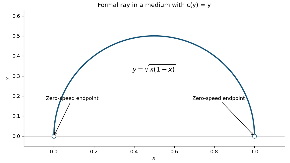
There is a necessary endpoint qualification. The speed is zero at the two stated endpoints. For any rectifiable path entering positive height, $ds/y\ge |dy|/y$, and its travel time diverges logarithmically on leaving or approaching height zero. Thus the semicircle is the formal interior ray, but there is no finite-time minimizer between the zero-speed endpoints. For endpoints at height $ϵ>0$ the circular ray has radius $\sqrt{1/4+{ϵ}^2}$ and finite travel time $2\mathrm{arsinh}(1/(2ϵ))$, which tends to infinity as $ϵ\downarrow 0$. This explains the intended semicircle as a limiting hyperbolic geodesic, without asserting finite travel time where $c=0$.

The expectation value of an observable is the mean outcome of repeated measurements on identically prepared systems in the normalized state. For a self-adjoint $Q$ it is real and equals $⟨\psi ,Q\psi ⟩$. Assume the state belongs to the domains needed for the second moments and the commutator below, so all these quantities exist.

For real $\lambda$, positivity of the squared norm givesThe commutator expectation is purely imaginary, so this is a real quadratic in $\lambda$. If $⟨P^2⟩>0$, its minimum is nonnegative exactly when its discriminant is nonpositive. If $⟨P^2⟩=0$, nonnegativity for all real $\lambda$ forces the linear coefficient to vanish, yielding the same conclusion. ThusReplace the observables by their centred versions $Q-⟨Q⟩I$, $P-⟨P⟩I$. Their commutator is unchanged, and their second moments are the variances $(\Delta Q{)}^2,(\Delta P{)}^2$. Taking square roots gives the Robertson uncertainty principleFor the quantum harmonic oscillator, $p=-i\hslash {\partial }_x$ gives $[x,p]\psi =i\hslash \psi$. The uncentred inequality above consequently gives $⟨x^2⟩⟨p^2⟩\ge {\hslash }^2/4$. The arithmetic-geometric mean inequality now yieldsThis is a bound for every normalized state of finite oscillator energy, not just an eigenstate. It is attained by the centred Gaussian ground state, for which $⟨p^2⟩=m^2{\omega }^2⟨x^2⟩$ and the uncertainty product equals $\hslash /2$.

The boundary circles intersect at $z=1$ and $z=i$: subtracting their equations gives $x+y=1$, and $x^2+y^2=1$ then gives these two points. Their intersection is the open lens in the first quadrant, bounded by the unit-circle arc from $1$ to $i$ and the corresponding lower-left arc of the circle centred at $1+i$.

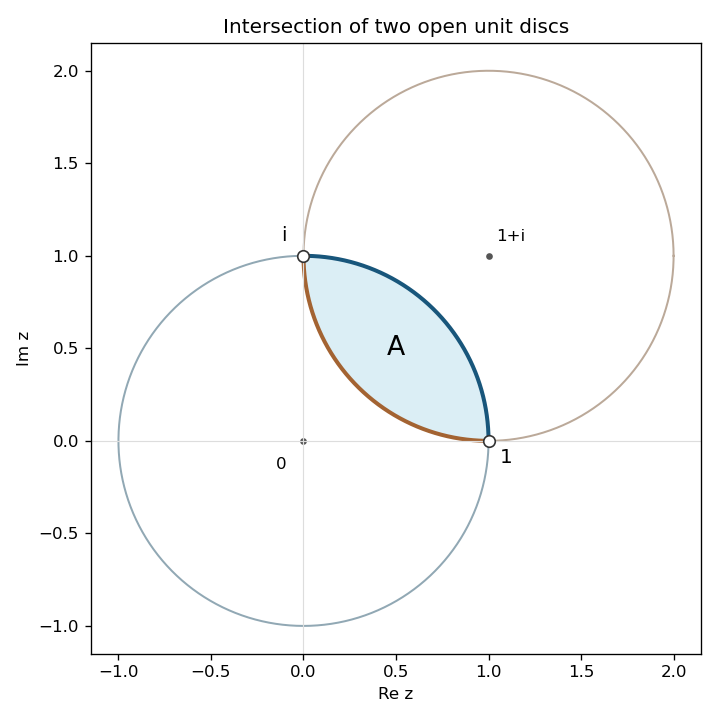
To construct a conformal map of a circular lens, apply the Möbius transformationIt sends the intersection points to zero and infinity, so both boundary circles become straight lines through zero. The boundary arc of the circle centred at zero maps to the ray of argument $-\pi /4$; the other arc maps to the ray of argument $+\pi /4$. For example, their arc midpoints $e^{i\pi /4}$ and $(1+i)-e^{i\pi /4}$ give these signs. The interior point $(1+i)/2$ maps to one, selecting the sector $-\pi /4<\arg \zeta <\pi /4$, not the complementary sector. As a Möbius bijection, $\zeta$ maps the whole lens onto that sector.

Squaring maps this sector bijectively onto the right half-plane: arguments double into $(-\pi /2,\pi /2)$, and the inverse is the unique square root with argument in $(-\pi /4,\pi /4)$. ThusThe derivative never vanishes inside the lens: $\zeta$ and its derivative are nonzero there. Finally use the Cayley transform between the half-plane and disk $w\mapsto (w-1)/(w+1)$. Since $|w-1|<|w+1|$ precisely when $\mathrm{Re}w>0$, it maps the right half-plane bijectively to the unit disc. The desired second map isThe denominator cannot vanish in the lens because $F(z)$ has positive real part. The maps send the centre-line test point $(1+i)/2$ to one and zero respectively.

For constant density, divide the incompressible Euler equations by $\rho$. The vector identity $(\mathbf{u}\cdot \nabla )\mathbf{u}=\nabla (|\mathbf{u}{|}^2/2)-\mathbf{u}\times \mathbf{\omega }$ converts them into ${\partial }_t\mathbf{u}=\mathbf{u}\times \mathbf{\omega }-\nabla (p/\rho +|\mathbf{u}{|}^2/2)$. Taking the curl eliminates the gradient. Expand the curl of the cross product, use $\nabla \cdot \mathbf{u}=0$ and $\nabla \cdot \mathbf{\omega }=0$, and obtainThis is the vorticity equation, including vortex stretching. Without constant density there would in general be an additional baroclinic term; the displayed source equations use the constant-density interpretation.

For the specified velocity, direct differentiation gives $\mathbf{\omega }=2\Omega (t)\mathbf{k}$. It is spatially uniform, while $(\mathbf{\omega }\cdot \nabla )\mathbf{u}=2\beta \mathbf{\omega }$. Thus ${\Omega }^{\prime }=2\beta \Omega$ andIf the positive $z$ direction agrees with the initial vorticity, $2\Omega (0)={\omega }_0$ as written in the question. For opposite rotation the initial component is signed and the vector has the corresponding minus sign.

For a material particle, $d(x^2+y^2)/dt=2x(-\beta x-\Omega y)+2y(-\beta y+\Omega x)=-2\beta (x^2+y^2)$, while $dz/dt=2\beta z$. The initial material circle therefore evolves intoThe azimuthal rotation changes the labels of points on the circle but not the circle as a set. Its counterclockwise circulation, viewed from positive $z$, isfor the positive-orientation convention. The strain contributes no tangential velocity. Thus circulation stays constant although vorticity grows and the enclosed material area shrinks, illustrating Kelvin's circulation theorem for a material loop in constant-density inviscid flow with no nonconservative body force.