The Robertson uncertainty principle bounds the product of the standard deviations of two observables in the same quantum state. For a normalized pure state and self-adjoint operators , write their expectation values and variances asand similarly for , where is the identity operator. The quantum uncertainties then obeyHere is the commutator, and every expectation value is taken in the same . These standard deviations describe the outcome spreads when and are measured on separate ensembles prepared in that same quantum state. They are not instrument errors or the change caused by a preceding measurement in quantum mechanics. The definition and bound are developed in Barton Zwiebach, Uncertainty Principle and Compatible Observables, 2013, §§1–2.
For unbounded self-adjoint operators, the operator domains matter. Assume , so that both second moments are finite; here means the second moment of the measured probability distribution, equal to , even if is undefined. To use the displayed operator commutator, also assume . Without these product-domain assumptions, the always meaningful version on uses as its right-hand side. These qualifications prevent a formal commutator identity from being applied to an inadmissible quantum state.
The brief proof is Cauchy-Schwarz inequality applied to and :The final equality uses self-adjointness and the product-domain assumptions. Thus a geometric statement about inner products becomes a constraint on experimental spreads. For nonzero , equality requires to be proportional with a purely imaginary proportionality factor; the equality case of the Heisenberg uncertainty relation turns this condition into a Gaussian wave packet.
The bound is useful because computing a single commutator and its expectation value can constrain two entire outcome distributions. Its right-hand side depends on the quantum state: the spin uncertainty state dependence example gives both a positive saturated bound and a zero bound for the same noncommuting observables. Robertson's paper, titled "The Uncertainty Principle", appeared on 1 July 1929 in Physical Review, volume 34, starting at page 163. [ref].
For self-adjoint operators and a normalized quantum state in their relevant product operator domains, put , , . With the inner product linear in its second entry, . The Cauchy-Schwarz inequality givesEquality holds exactly when are linearly dependent and . This includes either zero vector; if both vectors are nonzero it is equivalent to for real nonzero . Applying this inequality to the centred observables and gives the Robertson uncertainty principle.
A state saturating the uncertainty bound for a specified pair of quantum observables. The ground state of the quantum harmonic oscillator satisfies . Saturation is a property of the state and the chosen observables.
For a qubit, use the dimensionless Pauli matrices as observables , . Their Pauli matrix multiplication law givesThese observables have eigenvalues ; the physical spin components are , where is the reduced Planck constant, so their standard deviations acquire a factor .
In the computational basis, prepare , an eigenstate of with eigenvalue . Direct multiplication givesBoth Pauli measurements return and with equal probabilities, and the Robertson uncertainty principle is saturated: .
Instead prepare . Now the expectation values are , , so , . The Pauli measurement of is certain, and both sides of the bound vanish. The commutator is still nonzero as an operator: noncommuting observables do not guarantee a positive lower bound independent of the quantum state. This example is useful for distinguishing the algebra of the observables from the expectation values in a particular preparation.
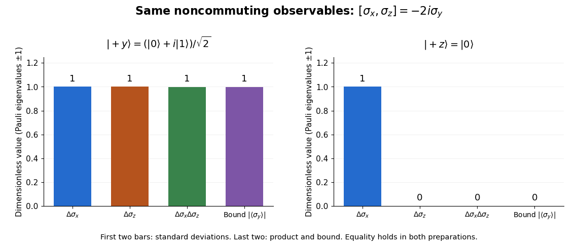
Pauli standard deviations, their product, and the Robertson bound in two preparations: the same noncommuting observables give bounds of one and zero
. Details. 
The Heisenberg uncertainty relation constrains the standard deviations of position and momentum in one preparation:On the real line, the position operator acts by multiplication, and the momentum operator is , with the reduced Planck constant. Their canonical commutation relation and the Robertson uncertainty principle give the bound on normalized quantum states satisfying the moment and product-domain assumptions above; Schwartz functions are a convenient sufficient class. Thus making a preparation more sharply localized in position forces a wider momentum distribution, even for ideal measurement in quantum mechanics.
An explicit saturating example is the normalized Gaussian wave packet, for ,The wavefunction is a probability amplitude; its squared magnitude is the probability density function, by the Born rule. That density is a normal distribution of mean zero and standard deviation , rather than a density whose width is read directly from the amplitude's exponent. With the unitary, negative-exponent convention for the Fourier transform, its momentum amplitude isThe Gaussian integral evaluates this Fourier transform. Consequently is another normal distribution, with mean zero and standard deviationFor example, in dimensionless units with , give . The Gaussian wave packets all saturate the same bound: narrowing one density broadens the other. More precisely, choose a reference length and set , ; then , and the plotted widths are and .
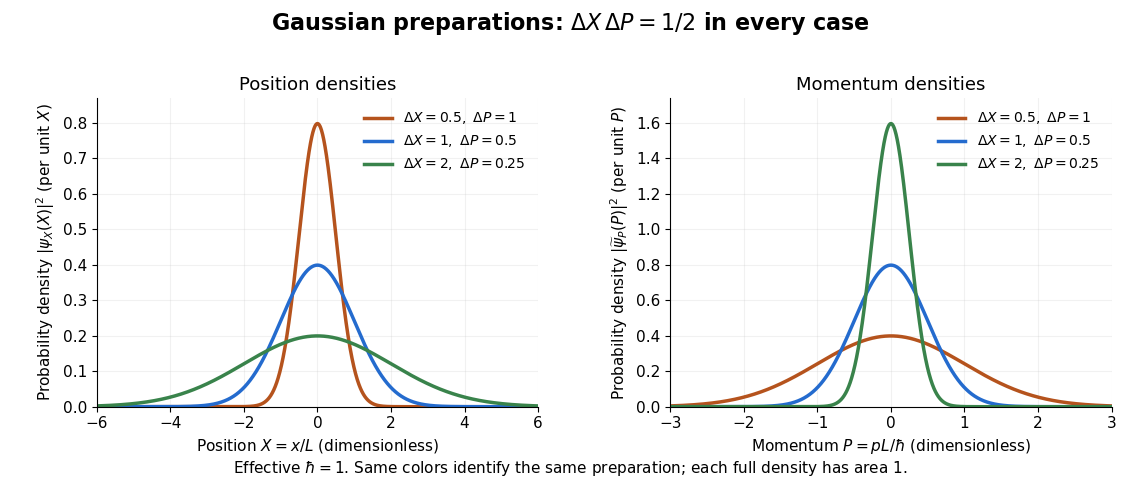
Position and momentum probability densities for three minimum-uncertainty Gaussian preparations: dimensionless widths 0.5, 1, and 2 in position give reciprocal momentum widths 1, 0.5, and 0.25
. Details. 
The Heisenberg uncertainty relation connects localization to the cost in kinetic energy. In a quantum harmonic oscillator with mass and angular frequency , the variance contribution to the expectation value of the energy is bounded using the arithmetic-geometric mean inequality:The mean-dependent contributions are nonnegative. The Gaussian eigenstate for a quadratic potential with and zero means reaches this ground state energy. This is why the tradeoff is more than a limitation on preparation: it predicts an unavoidable positive minimum energy.
Heisenberg's original article appeared in March 1927 as "Über den anschaulichen Inhalt der quantentheoretischen Kinematik und Mechanik", Zeitschrift für Physik 43, pp. 172–198. Its abstract discusses simultaneous imprecision of canonically conjugate quantities and explanatory thought experiments. The precise standard deviation formulation here distinguishes preparation spreads from a slogan about measurement disturbance. [ref].
The standard deviation of the momentum measurement distribution of a quantum state. A zero mean momentum need not imply zero momentum uncertainty. For a normalized state with finite moments, position and momentum uncertainties obey the Heisenberg uncertainty relation.
For uniform probability per volume in a sphere of radius , the radial probability density function is . Its root-mean-square radius is , whereas its scalar-radius standard deviation is . These are distinct from a fully specified quantum momentum uncertainty.
A normalized hard rectangular spatial wavefunction has a sinc-squared momentum density. Its central lobe has finite first-zero width , but its second momentum moment diverges. Thus that diffraction width is not a finite rms uncertainty. Smooth-edge states can have finite moments and satisfy the usual uncertainty inequality without this idealization.
Suppose each Cartesian coordinate of a particle of mass is supported in an interval of length , in dimensions. Popoviciu's inequality on variances gives , and the Heisenberg uncertainty relation gives . Since ,This is a rigorous but non-sharp confinement estimate. For a cubical infinite square well, separation of variables gives the stronger exact ground-state value . One must not identify a support length with a uniquely prescribed standard deviation or claim that the uncertainty estimate is the exact ground-state energy.
Preparation uncertainty describes the outcome spread intrinsic to a specified quantum state preparation. Operationally, prepare many copies of the same quantum state, measure position on one group and momentum on another, and estimate the two variances. Ideal measurements still have the spreads predicted by the Born rule. No earlier position measurement need occur in the momentum group. The Heisenberg uncertainty relation constrains these two distributions belonging to the same preparation.
Measurement backaction concerns how a particular measurement in quantum mechanics changes a quantum state. Instrument resolution concerns how its reported outcomes relate to the intended observable. Those questions require a model of the instrument and its interaction with the system. Substituting an instrument error and an induced change for and in the Heisenberg uncertainty relation does not follow from its proof. The practical value of preparation uncertainty is that it bounds achievable input spreads before any such instrument model is chosen.
Heisenberg's microscope is a thought experiment, not a report of a performed measurement. In Werner Heisenberg's Nobel lecture, The development of quantum mechanics, delivered on 11 December 1933, the imagined electron is illuminated with very short-wavelength light and observed through a high-resolution microscope. A scattered photon entering the observer's eye would, through Compton scattering, eject the electron from its original path. The passage challenges a classical trajectory picture; its microscope is hypothetical. The lecture date is 1933 even though the award is the Nobel Prize in Physics in 1932.[ref]
The Development of Quantum Mechanics by Werner Heisenberg. Nobel Lectures, Physics 1922–1941; Werner Heisenberg, The development of quantum mechanics, heading and printed pp. 291–292; text inspected in the Studyres transcription
The following idealized geometry makes the tradeoff visible. Let the collected light have wavelength and let the microscope objective accept outgoing directions within a half-angle about the vertical axis. Take transverse to that axis and hold the incoming photon momentum fixed. A diffraction-limited estimate of transverse resolution has scale . The unobserved outgoing direction admits transverse photon momentum components between approximately and , neglecting the angular variation of the scattered wavelength. By conservation of momentum, uncertainty in that component leaves uncertainty in the transverse recoil of the electron:Here is the Planck constant; the two symbols denote heuristic resolution and recoil scales, not the standard deviations in the Heisenberg uncertainty relation. Increasing the acceptance angle improves the estimated resolution while broadening the allowed recoil range. Numerical factors depend on the resolution criterion and angular distribution; this scaling argument cannot supply the sharp constant .
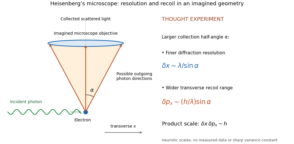
Heisenberg microscope thought experiment: an imagined scattering event and collection cone, with resolution and recoil scales rather than measured data
. Details. 
The thought experiment makes the interaction needed to obtain an image memorable. The preparation uncertainty theorem has broader use: it applies to the prepared quantum state even when the two observables are measured on separate copies. No claim that Werner Heisenberg built this gamma ray apparatus is needed to understand either argument.
A chirped Gaussian wave packet adds a quadratic quantum phase to the zero-mean Gaussian wave packet already evaluated above. Here and is a real dimensionless parameter. Its probability density function is unchanged for every , so and . Nevertheless, applying the momentum operator givesThe sign of the quantum covariance follows directly, without assigning a classical trajectory to the wavefunction:Here is a normalized symmetrized quantum covariance, analogous to a correlation coefficient. Positive gives positive , and reversing reverses while leaving both variances unchanged. In the negative-exponent Fourier transform convention used above, the momentum density isConsequently the quantum uncertainty product and the covariance matrix determinant tell different stories:Every member of this pure state family saturates the Robertson-Schrödinger uncertainty relation. Only saturates the Heisenberg uncertainty relation for this fixed pair of position and momentum axes. Thus being a Gaussian wave packet alone does not imply a minimum .
For a concrete comparison, choose a reference length , put , , and set . The choices all have , but give and , respectively. The two nonzero cases have and product ; all three covariance matrices have determinant .
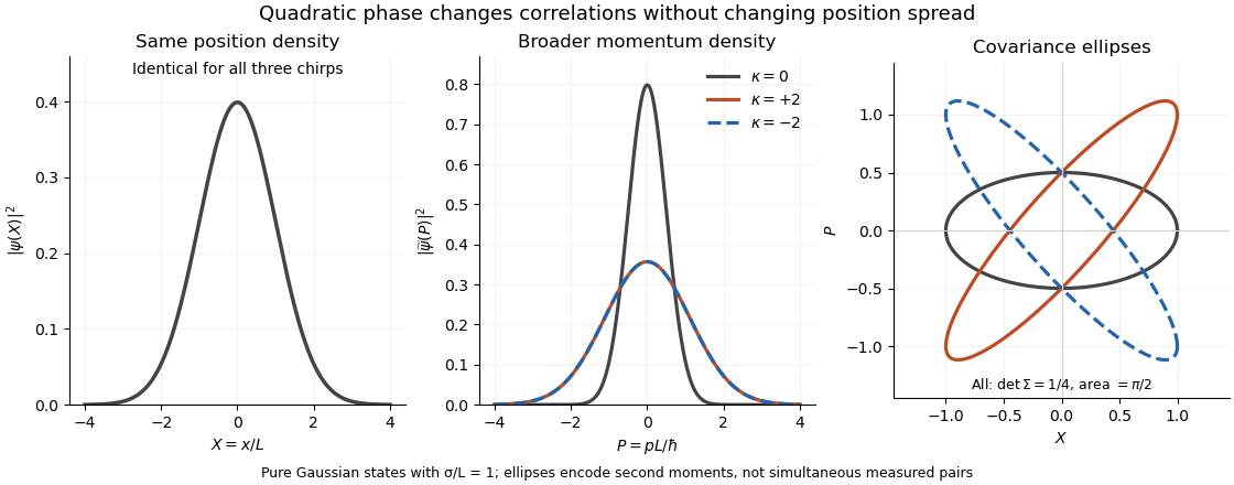
Quadratic phase preserves the position density but broadens the momentum density: opposite chirps tilt covariance ellipses in opposite directions while preserving their area
. Details. 
The phase space curves in the figure satisfy in the dimensionless coordinates, where . They display second moments, not observed simultaneous position and momentum pairs. Their common area is , although their coordinate projections differ.
This distinction is useful for predicting focusing. Under free particle evolution with mass , , soA negative chirp initially narrows the position distribution; positive chirp initially broadens it. For , the minimum occurs at and has variance . At that time the quantum covariance vanishes, and the unchanged momentum spread gives . The extra initial product was a usable position-momentum correlation, not extra measurement backaction.
For an admissible quantum state with zero position and momentum means, positivity of the squared norm for every real givesThe discriminant is nonpositive, hence . Subtracting the expectation values from the position operator and momentum operator extends this outline to nonzero means.
Equality in the Heisenberg uncertainty relation requires the centred vectors and to be imaginary scalar multiples, where , and are the expectation values. Thus, for some ,In the position representation, using the momentum operator turns this into a first-order differential equation, whose normalizable solutions areHence the quantum states saturating the Heisenberg uncertainty relation are these Gaussian wave packets, with arbitrary position and momentum means and global phase. Their width is . A Gaussian wave packet with an additional quadratic quantum phase need not saturate this product bound.
The Robertson-Schrödinger uncertainty relation keeps the real part discarded in the proof of the Robertson uncertainty principle. Write and . Their quantum covariance is . On the same finite-moment and product operator domains used above, the Cauchy-Schwarz inequality givesFor position and momentum, form the real, symmetrized covariance matrixA larger coordinatewise product can therefore encode a tilted covariance ellipse, rather than a larger determinant. This explains why the equality case of the Heisenberg uncertainty relation is more restrictive than equality in the Robertson-Schrödinger uncertainty relation.
For self-adjoint operators and an admissible pure state, the quantum covariance is the real, symmetrized second moment of two centered observables. The displayed expression uses their anticommutator; equivalently , which requires only the individual finite second moments. It reduces to ordinary covariance for commuting observables. For noncommuting observables, its definition does not assert that both have simultaneous sharp values drawn from a joint classical probability distribution.
Articles by others on the same topic
There are currently no matching articles.