
Past exam of the mathematics course of the University of Cambridge 2003 ia Paper 3 11A b Created 2026-09-24 Updated 2026-09-24
Past exam of the mathematics course of the University of Cambridge 2003 ia Paper 3 11A a Created 2026-09-24 Updated 2026-09-24
Past exam of the mathematics course of the University of Cambridge 2003 ia Paper 3 10A Solution Created 2026-09-24 Updated 2026-10-14
For the printed integration formula, must mean the Jacobian determinant of the inverse coordinate map:If instead one calls the forward Jacobian, its determinant is where the derivative is invertible. This convention distinction resolves the direction of the arrow in the printed wording.
To derive the change of variables formula, a small rectangular cell of side lengths maps under the inverse transformation, to first order, to a parallelepiped with edge vectors , , . Its volume is the absolute scalar triple product of those vectors:For a one-to-one continuously differentiable coordinate map with continuously differentiable inverse, summing these local volume contributions and taking the partition limit givesThe absolute value removes an orientation reversal; injectivity ensures that each volume element is counted once.
For positive semi-axes, take , , . The solid ellipsoid becomes the unit ball and the inverse Jacobian determinant is . ThusRotational symmetry gives equal integrals of over the ball. Their sum is the integral of , so spherical coordinates give . The Cartesian second moment of a solid ellipsoid is therefore
Past exam of the mathematics course of the University of Cambridge 2003 ia Paper 2 9F Solution Created 2026-09-24 Updated 2026-10-14
The inclusion-exclusion principle givesFor the coat problem, all permutations are equally likely. If a specified set of people gets its own coats, the other coats can be assigned in ways, so that intersection has probability . Taking the complement of the union of correct-coat events gives the derangement probabilityTo have exactly fixed coats, choose their recipients and derange all remaining coats. Thus the fixed point count of a uniform random permutation hasand zero probability outside this range. The empty permutation has , so the formula includes ; it also gives zero for , since a lone remaining coat cannot be misplaced.
For fixed , , and the exponential series givesThese are the probabilities of a Poisson distribution of mean one. The limit is for fixed , not for increasing with .
Past exam of the mathematics course of the University of Cambridge 2003 ia Paper 2 8D Solution Created 2026-09-24 Updated 2026-10-14
Differentiate the proposed first integral along the vector field:At , is conserved and the system is an inverted quartic oscillator phase portrait. Its equilibria are and . The Jacobian matrix isAt the origin its eigenvalues are . Moreover has a strict local minimum there, and its nearby positive contours are closed, so the origin is a genuine center equilibrium, not merely an inconclusive linear centre. The arrows circulate clockwise: on the positive -axis, . At either , the eigenvalues are , giving saddle equilibria. The stable eigendirection is , and the unstable one is .
The special energy level factors asBetween the two saddles, its left arc has and travels upward from to ; its right arc has and travels downward from to . These two heteroclinic orbits bound the central eye. Trajectories inside the eye are closed periodic orbits and do not tend to the centre as .
More explicitly, a level hasFor , its bounded central component is periodic, while its exterior components turn at and then escape. For , never vanishes and the two branches run from one vertical infinity to the other. Levels have only exterior nonconstant components, apart from the origin at .
On the upper outer separatrix, the branch arrives from positive infinity and approaches in forward infinite time; the branch leaves towards positive infinity. On the lower outer separatrix, the branch arrives from negative infinity and approaches , while the branch leaves towards negative infinity. Approaching a saddle along its stable manifold is exponential at rate . A trajectory close to but off a separatrix can spend a long time near the saddle before completing a periodic orbit or escaping.
The escape is finite-time blowup, not an asymptote at . On any escaping level, , so the remaining travel time is bounded by a convergent integral proportional to . Thus an outward upper branch has , ; an outward lower branch has , . The statement about approaching from infinity likewise refers to a finite past endpoint. Only equilibria, periodic trajectories and trajectories tending to saddles have a future defined for all time in this conservative portrait.
For small positive , the equilibria remain in place, but the origin's eigenvalues become , so it becomes a repelling focus. The saddles retain one eigenvalue of each sign, . Since , and its time integral is strictly positive on every nonconstant trajectory, trajectories cross -contours towards larger values. Near the centre this means outward spiralling. No nonconstant periodic orbit can remain, and the former saddle-to-saddle connections at equal are broken. Stable saddle trajectories approach from ; unstable ones depart into . Generic central trajectories eventually escape, while the exceptional stable saddle manifolds still approach their saddles.
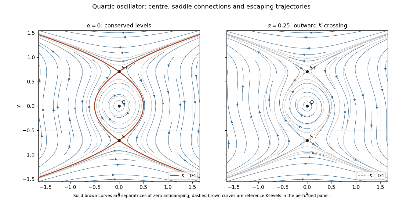
Conservative quartic phase portrait with heteroclinic separatrices, and outward contour crossing under small positive antidamping
. Details. 
Past exam of the mathematics course of the University of Cambridge 2003 ia Paper 2 7D ii Created 2026-09-24 Updated 2026-09-24
Past exam of the mathematics course of the University of Cambridge 2003 ia Paper 2 7D i Created 2026-09-24 Updated 2026-10-14
Past exam of the mathematics course of the University of Cambridge 2003 ia Paper 2 6D Solution Created 2026-09-24 Updated 2026-10-14
For two solutions , define the WronskianDifferentiate and substitute the second-order linear differential equation:Integration proves the Abel identity, including the identically zero case:For , this is on either interval excluding zero, since the integral uses . The coefficient singularity at zero must not be ignored.
Multiply the particular equation by and substitute the Frobenius solution . With , equating coefficients givesThe leading coefficient is nonzero, so the indicial equation is . Thus only are possible, and the recurrences below construct both.
For , , , and the recurrence reads , leaving free. For all later indices,This is an undetermined coefficient at Frobenius resonance; choosing selects a convenient even basis solution but is not forced by the differential equation.
For , all odd-indexed coefficients vanish andThe factorial denominators show convergence for every finite . Expanding the given hyperbolic functions directly yieldsConsequently the exponent-zero family is , and the normalized exponent-three solution is . This verifies the coefficient formulas and supplies two independent basis functions.
Finally and , soThis agrees with the Abel calculation. Its vanishing at zero does not contradict independence on regular intervals: the original equation is singular there.
Past exam of the mathematics course of the University of Cambridge 2003 ia Paper 2 5D b Created 2026-09-24 Updated 2026-09-24
Past exam of the mathematics course of the University of Cambridge 2003 ia Paper 2 5D a Created 2026-09-24 Updated 2026-09-24
Past exam of the mathematics course of the University of Cambridge 2003 ia Paper 2 4F Solution Created 2026-09-24 Updated 2026-10-14
The transformation is strictly increasing on , has range , and its inverse is . Therefore the cumulative distribution function isDifferentiation gives the probability density functionIts value at zero may be assigned arbitrarily without changing the distribution. There is no atom at zero or infinity. The expression is undefined at , but that event has probability zero under the continuous uniform distribution, so any convention there leaves the law unchanged. Finally , as required.
Past exam of the mathematics course of the University of Cambridge 2003 ia Paper 2 3F b Created 2026-09-24 Updated 2026-09-24
Past exam of the mathematics course of the University of Cambridge 2003 ia Paper 2 3F a Created 2026-09-24 Updated 2026-09-24
Past exam of the mathematics course of the University of Cambridge 2003 ia Paper 2 2D Solution Created 2026-09-24 Updated 2026-10-14
With , the central finite difference converts the decay equation toThe continuous ordinary differential equation has the general solution . The discrete linear recurrence is second order and requires two initial values, such as . Trying gives the characteristic equation of a linear recurrence . Its roots aresoThere are no repeated roots, and the same formula extends to negative integer if required.
To demonstrate the continuum limit, put . Then and , with . For ,uniformly, since . More precisely , giving an error on a fixed interval. Thus , selects the physical discrete mode and corresponds to .
The other root is a parasitic amplification root:For fixed , even and odd mesh points approach values differing by . Equivalently successive mesh values have a nonvanishing alternating jump despite their time separation tending to zero. This mode cannot converge uniformly to a continuous ODE solution; its limiting envelope also grows rather than decays.
For step-dependent initial data the precise result is the centered two-step discretization of exponential decay criterion:Sufficiency follows from the two uniformly bounded exponential envelopes on a fixed interval. Necessity follows from convergence at the adjacent points : , , and the coefficient formulas force , . In particular a nonzero but vanishing starting error is not excluded. Starting with the exact value gives and still converges on each fixed interval. The assertion about “remaining” solutions therefore concerns a fixed nonzero parasitic amplitude, not every nonzero step-dependent amplitude. The method is nevertheless not damping-stable for arbitrarily long times because .
Past exam of the mathematics course of the University of Cambridge 2003 ia Paper 2 1D ii Created 2026-09-24 Updated 2026-09-24
Past exam of the mathematics course of the University of Cambridge 2003 ia Paper 2 1D i Created 2026-09-24 Updated 2026-10-14
Past exam of the mathematics course of the University of Cambridge 2003 ia Paper 2 12F Solution Created 2026-09-24 Updated 2026-10-14
By rotational invariance, fix the first landing point at the north pole of a sphere of radius . A band of central angle and width has area . Dividing by total area gives the central angle between independent uniform sphere points densityand zero outside this range. The radius cancels.
Given the first pair's central angle , the third point can communicate with each of them exactly when it lies in that point's positive hemisphere. Choose their intersection line as a polar axis. Each hemisphere permits an azimuth interval of length , and the intervals' centres are separated by . Their overlap is a spherical lune of opening , with area . ThereforeThe union probability follows from inclusion-exclusion for two hemispheres:Thus the requested conditional answers are“Either” here is inclusive: a third ship linked to both is also linked to at least one.
For network connectivity, if the first pair is already linked, and the third must link to at least one of them. If , the first pair is not linked, and both must link through the third. Consequently the connectivity of three acute-angle sphere points isUsing and givesAngles exactly equal to the threshold have probability zero. Connectivity allows relaying and is weaker than requiring direct links between every pair.
Past exam of the mathematics course of the University of Cambridge 2003 ia Paper 2 11F Solution Created 2026-09-24 Updated 2026-10-14
An uneventful day leaves one aphid, a one-offspring day leaves the parent plus its offspring, and a two-offspring day leaves three aphids. Death leaves none. Thus the daily descendant counts are with probabilities , , , , respectively. The mean and probability generating function areIndependence across individuals and days makes the daily population a Galton-Watson process, with each surviving parent counted as one of the next day's descendants.
The standard Galton-Watson extinction fixed point result states that the eventual extinction probability of a branching process from one ancestor is the smallest root in of . Moreover a nondegenerate offspring law of mean at most one has extinction probability of a branching process one. Here, since , the fixed-point equation reduces towhich contains no . This proves laziness invariance of branching extinction: uneventful days change the timescale, not eventual extinction. The excluded case would keep one aphid forever.
If , the offspring mean is at most one. In this parameter range : if , then would imply . Thus the offspring law is not deterministically one, and the extinction criterion applies. Extinction is certain.
For the specified probabilities, the fixed-point equation factors asIts roots in are and , and the smaller root is the extinction probability of a branching process:
Past exam of the mathematics course of the University of Cambridge 2003 ia Paper 2 10F ii Created 2026-09-24 Updated 2026-09-24
Past exam of the mathematics course of the University of Cambridge 2003 ia Paper 2 10F i Created 2026-09-24 Updated 2026-09-24
There are unlisted articles, also show them or only show them.