
Maximal coupling Created 2026-09-24 Updated 2026-10-14
A maximal coupling of two probability distributions maximizes the agreement probability among all their couplings. Equivalently, it minimizes . The coupling characterization of total variation distance identifies the minimum mismatch with the total variation distance of the two marginal laws. The term maximal concerns agreement, rather than the size of a correlation coefficient or closeness in a geometric metric.
On a finite set, retain all common probability mass at equal pairs and match the excesses elsewhere. The explicit four-outcome example in coupling characterization of total variation distance realizes this construction and checks its marginal distributions. A maximal coupling need not be unique: different joint arrangements of the residual mass can have the same optimal mismatch.
Cantor's diagonal argument Created 2026-09-24 Updated 2026-10-14
Cantor's diagonal argument shows that the set of all infinite binary sequences is an uncountable set. Suppose a proposed enumeration is , where is coordinate of row . Construct a new binary sequence byIt differs from row at coordinate , for every . It is consequently absent from the entire proposed list, regardless of how that list was chosen. The failure of an enumeration of all binary sequences follows from this precise point of disagreement, rather than from a claim that the list looks too small.
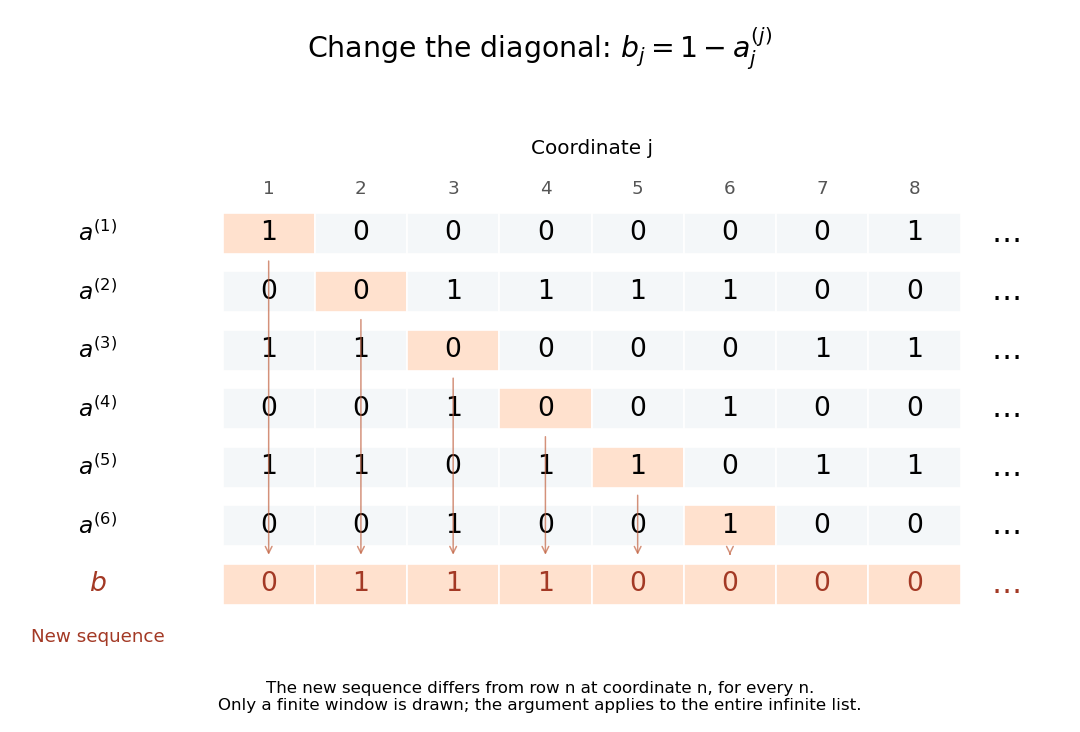
Flipping the nth coordinate of the nth row constructs a binary sequence missing from every proposed row
. Details. 
For the displayed window, the first six diagonal bits are , so the new sequence starts . The drawing shows only finitely many rows, but the rule defines every coordinate and excludes every row of an infinite list. This distinguishes the argument from the Cantor pairing function: that construction lists all pairs of finite indices, whereas this one concerns an entire infinite sequence as each object to be listed. Finite binary strings form a countable set; all infinite binary sequences do not.
The connection with power sets is exact: a subset corresponds to its indicator function, with a one in position exactly when . Changing the diagonal membership bit is the same mechanism as the Cantor's theorem construction . This reusable method turns a purported complete list into an explicit omitted object.
In his paper [ref]
https://onepagepapers.com/cantor-diagonal/read/. Cantor, Ueber eine elementare Frage der Mannigfaltigkeitslehre, pp. 75–78
, presented in 1891 and printed in the 1890–91 volume in 1892, Cantor uses infinite sequences of two symbols for the diagonal construction and then gives the broader comparison of cardinalities. The binary notation here is a modern presentation of that construction. Cantor pairing function Created 2026-09-24 Updated 2026-10-14
The Cantor pairing function is an explicit bijection between and , with the natural numbers numbered from zero:If , there are pairs on earlier diagonals, and the pair is at offset along diagonal . The formula therefore gives exactly the enumeration above. For example, .
Countable union of countable sets Created 2026-09-24 Updated 2026-10-03
Free-electron fraction during hydrogen--helium recombination Created 2026-09-24 Updated 2026-10-14
Saha ionization equation Created 2026-09-24 Updated 2026-10-14
Chemical equilibrium for givesafter neglecting the ion--atom mass difference in the translational prefactor.
Barotropic equation of state Created 2026-09-24 Updated 2026-10-05
A constant barotropic equation of state has . The cases and describe pressureless matter and radiation respectively.
Thermal decoupling in cosmology Created 2026-09-24 Updated 2026-09-24
A particle species thermally decouples when its interaction rate falls below the Hubble parameter. Its collisionless relativistic distribution subsequently redshifts with temperature proportional to , while annihilations among still-coupled species can heat the remaining plasma.
Effective number of relativistic degrees of freedom Created 2026-09-24 Updated 2026-10-06
The effective number of relativistic entropy degrees of freedom is defined byA relativistic bosonic degree of freedom contributes one, while a relativistic fermionic degree of freedom contributes when all species share a temperature.
Equation-of-state parameter Created 2026-09-24 Updated 2026-10-20
Photon-baryon fluid Created 2026-09-24 Updated 2026-09-28
Before recombination, frequent Thomson scattering couples photons, electrons, and baryons into an acoustic fluid.
Photon temperature multipole Created 2026-09-24 Updated 2026-09-24
Cosmic microwave background polarization Created 2026-09-24 Updated 2026-10-06
Thomson scattering of a local radiation quadrupole generates linear cosmic microwave background polarization. Its acoustic phase follows the photon velocity and is shifted by one quarter-period relative to the monopole temperature oscillation.
Slow-roll approximation Created 2026-09-24 Updated 2026-10-05
For a canonical scalar field with potential , slow roll reduces the field and Friedmann equations to
Inflaton Created 2026-09-24 Updated 2026-09-24
Positive semidefinite cone Created 2026-09-24 Updated 2026-10-05
The positive semidefinite matrices form a convex cone because nonnegative combinations preserve nonnegative quadratic forms.
Convex hull Created 2026-09-24 Updated 2026-10-18
The convex hull of a set consists of every finite convex combination of its points. It collects all choices obtainable by mixing the original choices with nonnegative weights summing to one. For in a real vector space,Equivalently this is the smallest convex set containing . Mixing two already mixed points produces another finite convex combination, so the displayed set is convex; every convex set containing must contain all these mixtures.[ref]
Convex Optimization by Stephen Boyd and Lieven Vandenberghe. §2.1.4, printed p. 24: convex hull and smallest containing convex set
In an original planar example, take four points , , , and four additional samples , , , . Their convex hull is the filled convex polygon , including its boundary. None of the samples is , butThe coefficients are nonnegative and sum to one, providing an explicit membership certificate. Geometrically, first form on the line segment , then mix . The additional interior samples do not enlarge the convex hull.
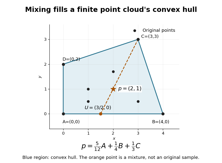

For a finite nonempty , the convex hull is the image of a probability simplex of weights under the linear map . The probability simplex is a compact set, and the map is continuous, so this convex hull is compact and closed. A one-point input stays one point; a collinear input stays in a line segment. Filling the convex hull does not necessarily produce a full-dimensional region.
The construction is useful whenever mixtures preserve the intended meaning of a choice. Mixing resource-allocation vectors, for example, interpolates their coordinate requirements. The convex hull describes the resulting feasible region. A coordinate-wise box can admit combinations that no mixture produces, as the outside-point certificate in linear optimization on a convex hull shows.
Second-order cone Created 2026-09-24 Updated 2026-10-14
Euclidean projection onto a convex set Created 2026-09-24 Updated 2026-10-14
For a nonempty closed convex subset of a finite-dimensional inner-product space, is the unique point of minimizing .
This closest-point map is the metric projection onto a closed convex set. Repeated projections onto several sets form the separate projections onto convex sets method.
Extreme point Created 2026-09-24 Updated 2026-10-18
An extreme point of a convex set is a point that cannot be made by genuinely mixing two different points of the set. For a convex set in a real vector space, the condition on isThus lies on no open line segment between two distinct points of . It is enough to exclude midpoint representations: if lies inside a line segment, two nearby points on opposite sides have midpoint .[ref]
Convex geometry (BME course BMETE94AM22). §6, Definition 6.6, printed p. 37: extremal points of closed convex sets
The square has just four extreme points, at . In a convex combination giving a corner, each coordinate is already at its largest or smallest allowed value, forcing both input points to agree with that corner. In contrast, the boundary point is not extreme:It is the midpoint of two other points on the same edge. An interior point also admits a small line segment through it.
The unit disk has a different shape: every point on its unit circle is extreme. For a unit vector , the Cauchy-Schwarz inequality givesand equality is possible only at . If a convex combination equals , applying this linear functional forces both ingredients to attain that equality. Both must therefore be . Extremality need not look like a sharp corner.
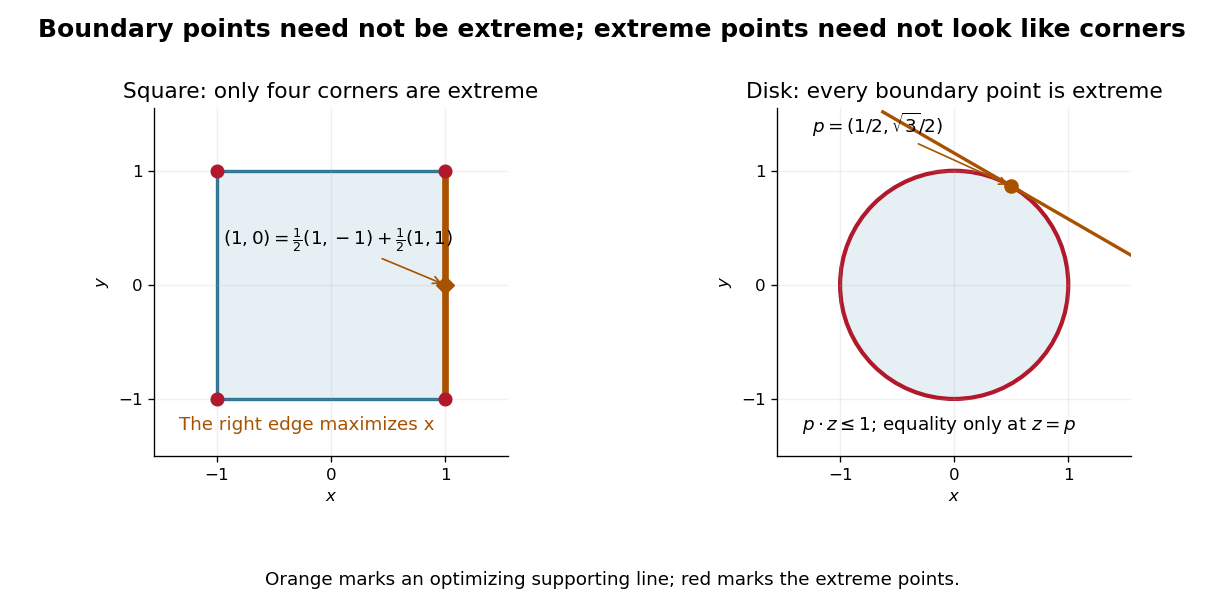

These points help describe all allowable mixtures. Every is a convex combination of its four corners, with the weight on equal to . For the unit disk, write , with and a unit vector; at zero choose any . ThenTwo extreme points suffice for that mixture. The Krein-Milman theorem gives a much broader reconstruction: a nonempty compact convex set in a locally convex space whose topology is Hausdorff is the closed convex hull of its extreme points.
Mark Krein and David Milman published their reconstruction theorem in 1940. Milman's colleagues describe that result and its subsequent use as a method of representing convex sets through their extreme points.[ref]
David Milman (1912–1982) by Israel Gohberg and others. David Milman (1912–1982), printed p. 4: 1940 collaboration with M. G. Krein, the reconstruction theorem and subsequent method; citation 3 refers to their original paper
There are unlisted articles, also show them or only show them.