
A free-fall timescale estimate follows from :Falling to a central point mass gives the more precise factor , or ; a distributed star changes an order-one coefficient. For any spherical mass distribution with radius ,The inequality is strict for an extended star; equality is approached by a thin shell at . For an monatomic gas the virial theorem is , so half the gravitational potential energy released by contraction heats the star and half can be radiated. The Kelvin-Helmholtz cooling time is therefore of orderA uniform-density model gives . The given bound fixes a scale, rather than an exact contraction history; both estimates are far shorter than the Sun's main-sequence lifetime.
A thin spherical shell has outward pressure force and inward gravitational force . Hydrostatic equilibrium requiresA uniform-density solar model gives , , and after integration from to zero,Thus the appropriate orders of magnitude are – and . The uniform-density approximation underestimates the actual central pressure because the Sun is centrally concentrated. Radiation pressure is neglected in applying the ideal gas law.
Adopt the approximate mass-luminosity relation and equal available fuel fractions. The main-sequence lifetime then scales as , givingUsing an exponent instead gives about and years; these are model-dependent estimates. At the Newtonian gravitational potential energy released from infinity is . Half remains as kinetic energy in a circular orbit, so the radiatable binding energy is :Using the whole potential energy loss would give , which does not subtract the final kinetic energy. A fully relativistic calculation for a nonrotating black hole gives . When the surviving star exhausts hydrogen burning, it expands off the main sequence and can fill its Roche lobe. Binary mass transfer to the black hole can form an accretion disk and an X-ray binary; unstable binary mass transfer may instead produce a common envelope. This is conditional on the binary star remaining bound after the first remnant forms. The supplied black hole endpoint is an assumption, not a universal outcome for an isolated star.
Assume a circular orbit and an orbital inclination , as appropriate for a simple eclipsing binary estimate. At quadrature the two radial velocities are opposite and equal to the orbital speeds. The more massive component has the smaller amplitude. With the centre of mass as origin,Thus , and Kepler's third law givesThe orbital plane contains the observer's line of sight; at quadrature the two velocities point towards and away from that observer, as labelled in the original schematic below. For an elliptic orbit, the measured amplitudes instead give ; the numerical answer requires the circular assumption.
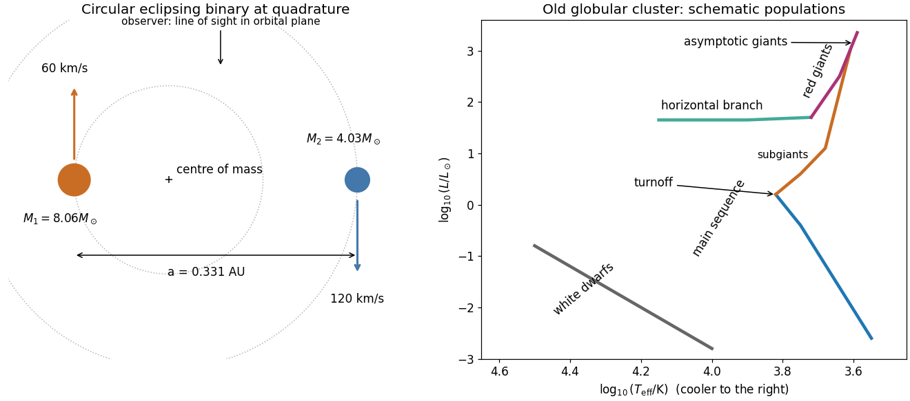

Kepler's third law for two point masses in a Newtonian gravitational field isHere is the semimajor axis of their relative orbit, the orbital period and the gravitational constant. Equivalently , to the accuracy with which these astronomical units normalize the solar mass.
Shrink the positive outer contour to the branch cut . On its upper bank the chosen branch of a multivalued function has and on the lower bank it has the negative of this value. The upper bank runs from to , and the lower bank runs from to . The endpoint circles contribute and vanish. HenceThe change of variables independently reduces the result to the integral of over .
Use the branch cut and the branch of a multivalued function normalized by . The Laurent series from the preceding solution has coefficient . Consequently every sufficiently large positively oriented circle givesAlthough grows cubically, its other Laurent series terms have zero contour integral. Choosing the opposite branch of a multivalued function reverses the sign; neither the branch of a multivalued function nor the orientation can be omitted from the answer.
The square root produces branch points at , with local behaviour proportional to . One branch cut can join them along . Another choice uses the two rays . Each choice prevents a loop from enclosing just one branch point within a single-valued domain. For the finite-segment choice fix at infinity. Infinity is then a pole of order three, not a branch point, since
Put , so , and . The contour integral isThe enclosed poles are and . For the rational function displayed without the prefactor , the residue at zero is and the two other residues sum to . Therefore the residue theorem givesA useful independent check is the Fourier series ; only its constant and third Fourier coefficients survive.
Cauchy's integral theorem states that a holomorphic function on a simply connected open region has zero contour integral around every closed piecewise smooth contour in that region. More generally the same holds for a contour homologous to zero in its domain of holomorphy. Having no singularity on the curve alone is insufficient: has a nonzero contour integral around the unit circle.
If , then and its residue at zero is . The circle encloses zero and no other finite singularity. Thus the residue theorem givesfor positive orientation.
For a positively oriented circle of any radius , the residue theorem givesOnly the coefficient in the Laurent series contributes. Reversing the orientation changes the sign.
For , is holomorphic at every finite nonzero point. At zero its Laurent series has infinitely many negative powers, so zero is an essential singularity. If the Riemann sphere is included, has a pole of order at , so infinity is a pole of order .
Choose a continuous branch of a multivalued function of the complex logarithm on a simply connected region avoiding zero. ThenAlternatively and , verifying the Cauchy-Riemann equations. The holomorphy is local to a chosen branch of a multivalued function: increasing by multiplies by , so this is not a single-valued holomorphic function on the whole punctured plane.
The chain rule in polar coordinates gives and , with analogous expressions for . Substituting the Cauchy-Riemann equations givesThe restriction excludes the coordinate singularity at the origin.
Set and . Direct differentiation givesTheir sum vanishes, proving that is a harmonic function. More generally the Cauchy-Riemann equations give and ; the mixed partial derivatives commute because a holomorphic function is smooth. Since , a harmonic conjugate and the resulting holomorphic function areThese expressions also verify the Cauchy-Riemann equations directly.
A complex derivative computed along the real and imaginary directions gives . Equality yields the Cauchy-Riemann equationsThe gradients satisfy . Since a gradient is normal to a regular level set, the two families meet at right angles by orthogonality wherever . At a critical point the regular-curve argument fails: for both gradients vanish at zero, so the assertion requires this qualification.
Since , increasing hunting effort moves leftward on these diagrams. The first stability threshold corresponds toAbove this removal rate, a sufficiently small grey population can be eliminated while reds recover. Until the second threshold, however, the system is bistable: an initially large grey population can still win, so the history and initial abundances matter. The second threshold isAbove it, any positive red population recovers and the grey population tends to zero, regardless of its initial abundance in this deterministic model. This threshold is smaller than , so competition from surviving reds can make eradication possible with less removal than would be necessary to suppress grey growth without competitors. If , part (a)(iii) supplies the simpler competitor-independent extinction bound. These are model predictions about long-term dynamics; neither finite-time extinction nor uncertainty in ecological parameters is encoded in the equations.
Write . The physically nonnegative branches, omitting , areOn both bifurcation diagrams, draw solid for and dashed for ; draw dashed for and solid for . The coexistence branch is dashed throughout its interior because it is a saddle point. It connects at to at , through two transcritical bifurcations when the branches are continued mathematically beyond the nonnegative quadrant.
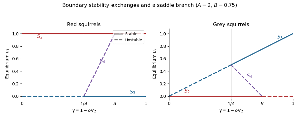
Stable boundary populations and the unstable coexistence threshold
. Original bifurcation diagrams for , . Solid branches are asymptotically stable, dashed branches unstable. The physically admissible coexistence branch joins the grey-only branch at to the red-only branch at . Details.
There are unlisted articles, also show them or only show them.