
Under , , , the thresholds are ordered . As decreases from one, first becomes stable atFor , both boundary equilibria are stable, and the positive coexistence point is a saddle point. Its stable manifold is the separatrix between their basins of attraction. For every fixed , a sufficiently small positive lies in the red-survival basin. To justify the quantifier beyond a neighborhood of , start on the red-only axis: its logistic equation approaches . Continuous dependence over the finite time needed to enter a stable neighborhood shows that sufficiently small positive initial grey populations do so as well.
At the second threshold, meets . For , is a saddle point, its stable manifold is the grey-only axis, and there is no positive coexistence equilibrium. Boundedness and the same Bendixson-Dulac theorem argument rule out an interior cycle. Consequently every initial state with and approaches . This is the removal regime that eliminates grey squirrels regardless of their initial abundance. At threshold equality linearization is nonhyperbolic; the strict parameter intervals above avoid inferring stability from a zero eigenvalue.
The non-axis nullclines are and . For , , the first has intercepts and the second has . Their axis intercept order rules out a positive intersection. Below the first line increases and above it decreases; below the second increases and above it decreases. Thus is a saddle point and is stable.
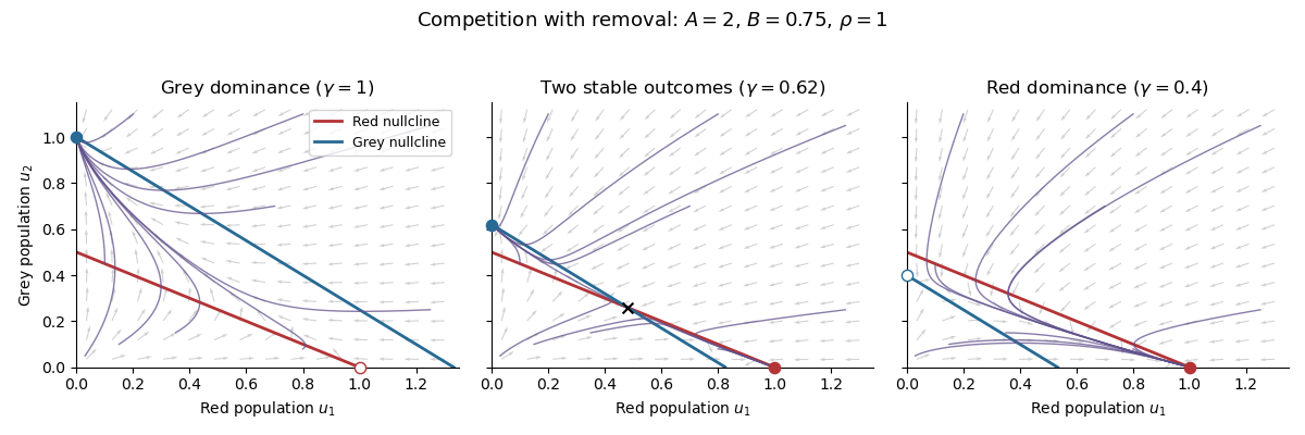

For strictly positive initial populations, both coordinates stay positive and are bounded above by their individual logistic equations. There are no interior periodic orbits: the Dulac function makes the divergence of the multiplied vector field , so the Bendixson-Dulac theorem applies. The stable manifold of is the invariant red-only axis, and is repelling. The phase portrait, or the Poincaré-Bendixson theorem with these boundary directions, therefore givesThe qualification matters: a grey population identically absent cannot drive extinction. In dimensional variables, positive grey presence leads to , in this no-hunting case.
Abbreviate , . The coordinate factors immediately give the three boundary equilibria . The Jacobian matrix isAt , the eigenvalues are , so it is a repelling equilibrium. At the other two points, triangularity givesTherefore is asymptotically stable for and a saddle point for ; is asymptotically stable for and a saddle point for . Equality gives a zero eigenvalue, so linearization alone is inconclusive there.
For later use, the coexistence point is physically positive exactly when if , or if . Its stability is as supplied in the question. If the displayed formula for does not apply: when also , the coincident non-axis nullclines give a whole segment of equilibria.
The nonnegative quadrant is invariant because both right-hand sides have the corresponding population as a factor. There . The differential inequality, or the Gronwall inequality, givesBiologically means : per-capita removal exceeds even the grey squirrels' maximum uncrowded growth rate. Competition can only strengthen the decline.
Since , division of the equations by givesThus the dimensionless parameters areEach is a ratio of quantities with matching units. In particular can be negative even though every original model parameter is positive.
The terms give intrinsic per-capita population growth. The terms model intraspecific crowding in a logistic equation, while model interspecific competition. Here is the single-species carrying capacity, and measures the competitive effect of one unit of species relative to one unit of species in that species' crowding term. The last term is per-capita removal of grey squirrels: constant effort, rather than a constant number removed per unit time.
When , expand the denominator:The leading term is ordinary Galilean velocity addition. When both from below, the exact formula instead gives , rather than . Indeed, writing , , we have whenever .
Using and the hyperbolic tangent addition identity,Consequently the relativistic velocity addition rule is
For the collinear boosts specified in the question, multiplication of the two -by- blocks and the hyperbolic addition formulas giveThus the resulting rapidity is . Collinearity matters: boosts in different spatial directions do not in general combine into a pure boost of this form.
For increasing parameter along a future-directed timelike curve, the elapsed proper time isor when coordinate time is the parameter. A Lorentz transformation satisfies , so replacing by leaves the expression under the square root unchanged. Hence the integral is invariant. A monotone change of path parameter also leaves it unchanged by the ordinary substitution rule.
Use the Minkowski metric and coordinates . At a point, a smooth path is timelike if its tangent is a timelike vector, here meaning . It is lightlike if its tangent is a null vector: the same expression is zero and the tangent is nonzero. In these coordinates, a future-directed timelike tangent has spatial speed less than ; a lightlike tangent has speed .
Take a minimum spanning tree , for example one constructed by Kruskal's algorithm. Fix and let be a longest edge of the tree's unique path. Deleting partitions into two components separating and . Any alternative path crosses this graph cut. If all of its edges were shorter than , a crossing edge would let us replace by , producing a spanning tree of smaller total length. This contradicts minimality of .
Therefore every competing path has an edge at least as long as , and the tree path solves the bottleneck shortest path problem. The same minimum spanning tree works simultaneously for every ; this is the minimax path property of a minimum spanning tree.
Let be the smallest threshold for which the edges of length at most connect to . This is exactly the optimum value of the bottleneck shortest path problem. While any edge longer than is being processed, every edge of some threshold- route is still present, because shorter edges have not yet been processed. Thus all edges longer than are deleted. The final path from part (i) consequently has maximum edge length at most . It cannot have a smaller maximum by the definition of , proving optimality. Ties in edge ordering do not affect this argument.
There is an index slip in the source: starting with and performing steps produces the final graph . Write for that final graph. The literal assertion for can fail: take a triangle with , , . Before the final step the extra edge remains; only the final deletion removes it.
The invariant is that and remain connected. Choose a simple graph path in . If an edge of did not lie in , then at its processing time was still present and avoided that edge. The algorithm would therefore have deleted it, a contradiction. Thus every edge of lies in . The final graph is precisely an path and possibly isolated vertices.
Starting from , the initial tentative distances to are . Finalize next. Its edges improve these to , , and . No subsequent relaxation improves them. Hence one shortest-path tree isThese values follow either by completing Dijkstra's algorithm in the order , or by observing that any internal vertex on a simple route adds to the direct-edge cost: only the internal vertex can reduce it.
For Dijkstra's algorithm, initialize and for other vertices, with no predecessor initially. Repeatedly select an unfinalized vertex of least tentative distance, finalize it, and relax each edge : if , replace by that value and set the predecessor of to . Continue until all vertices are finalized. The predecessor edges form the shortest-path tree.
To justify finalization, consider a supposedly shorter route to the next selected vertex. Its first unfinalized vertex is preceded by a finalized one, whose relaxation would already have offered a tentative distance no greater than the length of that route's prefix. Nonnegative remaining lengths would contradict the selected vertex's minimal tentative label. Thus final labels are the true shortest distances. Strictly positive lengths also make predecessors have smaller distances, ruling out predecessor cycles in a graph.
A shortest-path tree rooted at is a spanning tree such that, for every vertex , the unique graph path in has minimum total edge length among all graph paths in . The objective is the sum of the lengths along each route, not the sum of all the tree's edge lengths.
A spanning tree of the connected graph is a subgraph containing every vertex, connected and without cycles in a graph. Equivalently, between every pair of vertices it has exactly one graph path. For a finite graph with vertices, it has edges.
In the space of tempered distributions, this Fourier transform convention gives and . ThereforeThe constant distribution and the Dirac delta distribution are linearly independent: testing away from zero first determines the constant coefficient, and then testing at zero determines the delta coefficient. Hence and , giving
At zero, the Fourier transform is , so . In particular and . The Fourier inversion theorem at zero also givesEquating the two values yields . Since the explicit normalized Gaussian function in part (i) has , here .
There are unlisted articles, also show them or only show them.