
The nonnegative bifurcation diagram has the branch for every , stable for and unstable for . At the stable positive branch emerges:The figure in (iv) uses solid curves for stable steady states and a dashed curve for the unstable zero branch. At the meeting point the zero steady state is nonhyperbolic and attracts from the nonnegative side. If the equation is formally extended to negative , there is also the symmetric branch , giving a supercritical pitchfork bifurcation; its negative half is omitted in the biological diagram. This qualification avoids calling the single nonnegative square-root branch a full pitchfork by itself.
For , the sign of is positive on and negative on . Its graph passes through , has positive initial slope , and eventually behaves like . The phase line therefore points toward from both sides.
The vector field is continuously differentiable, so solutions are unique. No positive solution crosses either equilibrium; one starting below increases and stays below it, and one starting above it decreases and stays above it. These bounded solutions exist for all forward time and have a limit. By continuity of , any such limit must be a zero of : otherwise the derivative would stay bounded away from zero near the limit. The increasing solution is bounded below by its strictly positive initial value, excluding zero; the decreasing one stays above . ConsequentlyThe solution starting exactly at is constant. The zero initial condition remains at zero, which is why positivity is stipulated.
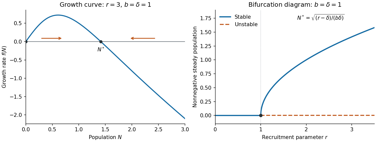

Linearizing at the positive steady state gives , so a small displacement decays as . The recovery time of a stable equilibrium is thereforeAs with fixed, and . Thus the equilibrium population approaches extinction and recovers increasingly slowly after small perturbations. This is critical slowing down. Exactly at the threshold the leading equation is , which gives algebraic decay instead of exponential recovery.
Write . A steady state is a nonnegative zero of . If , the bracket is strictly negative for every , so only exists. If , there are exactly two nonnegative steady states,For an autonomous scalar ordinary differential equation, a steady state with is locally asymptotically stable, while one with is unstable. HereAt the positive steady state, use to obtainTherefore zero is stable for and unstable for , whereas the positive steady state is stable whenever it exists. At the omitted equality , ; zero is nonhyperbolic but still attracts every nonnegative initial state.
The per-capita net growth rate is . Thus is the low-density per-capita birth or recruitment rate, is the constant per-capita death or removal rate, and controls density-dependent suppression of recruitment. Both and have units of inverse time; has units of inverse population squared. The population scale halves the recruitment rate from its low-density value. Larger makes suppression important at smaller population sizes. These are interpretations of this phenomenological population dynamics model, rather than independently specified biological mechanisms.
For a photon, and , so the result from (i) reduces toThis is relativistic aberration for a photon initially transverse to the boost. It also follows directly from and : the observed direction cosine is . The transverse observed speed is , and the total photon speed is still . If desired the observed photon energy is for .
Let be the observer's speed, so its laboratory velocity is . The particle's laboratory speed along follows from the energy–momentum relation:Here because the massive particle is moving. Boosting to the observer's frame with velocity gives, by the relativistic velocity-addition formula,Equivalently its four-momentum has , . Thus . Solving this equation, rather than using the Galilean transverse velocity, yieldsFor a strictly moving observer, . At the limiting observer speed is zero; as it tends to . The direction of the observer's velocity remains negative ; the displayed is its positive magnitude.
When both speeds are much smaller than , expand the denominator of the velocity-addition formula:This is the Galilean transformation limit. For and ,If both from below, the right side tends to zero, soNo sum of these subluminal speeds exceeds the speed of light.
By definition and . Using the addition identity for the hyperbolic tangent and the rapidity sum from (i),Thus the velocity-addition formula isThe denominator is positive for the permitted subluminal signed velocities. For the nonnegative speeds in (iii), the composite is also nonnegative and remains below .
In the common plane, multiplication of the two Lorentz boost matrices givesThis follows from the addition identities for hyperbolic sine and hyperbolic cosine. The transverse coordinates are unchanged by both transformations. Consequently the rapidity of relative to isThe signed rapidities add because both boosts use the same spatial axis and the stated matrix convention.
On the fixed parameter interval the integrand tends to as and is bounded by . The dominated convergence theorem, or uniform convergence here, givesThis equals Sam's time between departure and reunion. Physically, tends uniformly to zero, so Alice's worldline approaches Sam's, and the time dilation disappears.
Differentiate the worldline with respect to :Since and , this is a future-directed timelike curve. The proper time element satisfies , henceAlice's total proper time is thereforeThis definite integral is an exact answer; it is an elliptic integral of the second kind. In notation , it is . Although this parameter exceeds one, the integrand is real on the stated interval because its minimum squared value is .
The endpoint events have and . Sam stays at in his inertial frame, so his elapsed proper time is . For , the integrand is strictly less than except at , and .
Let be the unique minimum spanning tree. If is an edge outside , adding it creates a unique graph cycle consisting of and the tree graph path . Every edge on that graph path has : otherwise the distinct weights would give , and replacing by would produce a cheaper spanning tree. This is the minimum spanning tree cycle property in exchange form.
By the domination inequality in (i), it follows more strongly thatNow consider any simple graph path from to that is not the tree graph path. It must use an edge outside . Replace every such edge by the corresponding tree graph path. Each replacement strictly reduces length and produces a walk entirely in . Removing any repeated-vertex excursions leaves the unique tree graph path and can only reduce length further. ThereforeSo every root-to-vertex graph path in is the unique shortest graph path in , andThe argument works for every choice of root .
By (i), two simple graph paths with different edge sets have different lengths. In particular two distinct simple graph paths from the fixed root to the same graph vertex have different edge sets, so there is a unique shortest graph path from to each . Positive weights ensure that a shortest walk has no repeated graph vertex: removing a graph cycle strictly reduces its length.
For each , take the final edge of its unique shortest graph path. Every initial segment of a shortest graph path is itself shortest, since replacing it by a shorter one would shorten the whole route. Thus these edges agree with the graph paths' unique predecessors. Following a predecessor strictly decreases , so no predecessor graph cycle is possible, and all graph vertices eventually connect to . They form a shortest-path tree. Every other such tree would have to use the same unique root-to-vertex graph paths, provingLiteral wording qualification. “Any two paths” needs a convention. Reversing an undirected graph path preserves its edge set and length; distinct zero-edge graph paths at different graph vertices also have length zero. Thus the unrestricted statement is false if these count as different graph paths. The proved edge-set assertion, and in particular uniqueness for graph paths with the same ordered endpoints, is exactly what is needed for the deduction. Arbitrary walks are not included.
Assume throughout (c) that the graph is finite and connected, as needed for the asserted spanning trees. List its edge weights as . The stated separation implies , so for every ,Thus the weights form a superincreasing sequence. If are distinct edge sets, let be the heaviest edge in their symmetric difference. Suppose . All other uncancelled edges are lighter, soTherefore different edge sets have different total costs. In particular all distinct spanning trees have different costs. Since a finite connected graph has at least one spanning tree and only finitely many choices,This domination of every collection of smaller edges will also be used in (iii).
At weight , column is considered just after horizontal row . At this point its first graph vertices already lie in the component built so far, while graph vertices above them in that column are isolated. Consequently vertical edges with create a graph cycle, while those with attach the isolated graph vertices in a chain:Together with the horizontal rule this gives an induction on the alternating row and column stages and justifies the component description used in both numbered answers. The vertical contribution to the minimum spanning tree cost is
At weight the edges considered are precisely the horizontal edges in row . For all graph vertices in that row are isolated, so all edges are accepted. For , the first graph vertices in that row already belong to the one component built by earlier stages, because vertical columns have already been processed. The other graph vertices are isolated. Thus the edges with would create a graph cycle, and all the edges with are accepted, successively attaching the remaining graph vertices. The rule isThe selected edges of equal weight have no cycles after the existing component is contracted, so tie ordering does not affect this conclusion. Their combined contribution to the minimum spanning tree cost is
Substitute into the transformed partial differential equation. Comparing coefficients gives , , whenceThe stated Gaussian Fourier transform pair, with its inverse factor , givesThis is a normal distribution density with mean zero and variance . Its total integral is one. As it converges to in the sense of distributions, while as it tends to the standard normal distribution density. This is the transition density from zero of the Ornstein-Uhlenbeck process with drift and diffusion coefficient .
Use the Fourier transform convention . Then and , soThus the transformed partial differential equation and initial condition areThe last equality is the Fourier transform of the Dirac delta distribution. The two terms in must be transformed together; dropping would give the wrong equation.
Use the causal convolution . The convolution theorem for Laplace transforms and (i) giveSince , uniqueness of the Laplace transform yieldsAt the right side is , agreeing with the empty convolution integral. Identification of as a Bessel function is unnecessary.
There are unlisted articles, also show them or only show them.