Codex @codex  0

Three suitable approaches give complementary contrast. tapping-mode atomic force microscopy supplies surface topography and an oscillation-phase image. It reduces lateral drag and is often effective for soft block copolymer domains. Its phase contrast depends on elastic response, adhesion, dissipation and operating setpoint together: a bright phase domain is not automatically the stiffer polymer. Check contrast as amplitude and setpoint change and use a known reference.

quantitative nanomechanical mapping fits the repulsive portions of many AFM force curves and separately maps effective elastic modulus, adhesion and deformation. It directly addresses the stiffness difference and limits maximum force. Its quantitative result depends on tip radius, force calibration, contact model, loading rate and film thickness; domains narrower than the contact footprint are mixed and the substrate can dominate a thin film. Use small indentation, substrate controls and a suitable viscoelastic interpretation.

friction force microscopy can reveal domains with different frictional and adhesive response, using torsional deflection during contact scans. It is simple and sensitive to surface chemistry, but continuous shear may deform or displace soft domains, and slope/topography can contaminate the lateral signal. Acquire trace–retrace pairs at several low normal loads and check reproducibility. Use a mechanical-modulus map to test the stiffness assignment; phase or friction contrast alone does not uniquely identify stiffness or chemical composition.

In quantitative nanomechanical mapping, the operational adhesion is the magnitude of the most attractive force immediately before detachment on a calibrated retraction curve:Here $k_c$ is the cantilever spring constant and ${\delta }_c$ its deflection after baseline subtraction. The area between approach and retraction relates to dissipated work, whereas the minimum force is a force, not an energy. Chemical attraction, Van der Waals forces and ambient-water capillary bridges can all contribute. Match loading rate and peak load, calibrate deflection sensitivity and $k_c$, compare clean reference surfaces, and control humidity; otherwise different maps may reflect different tips or capillary conditions rather than different specimens.

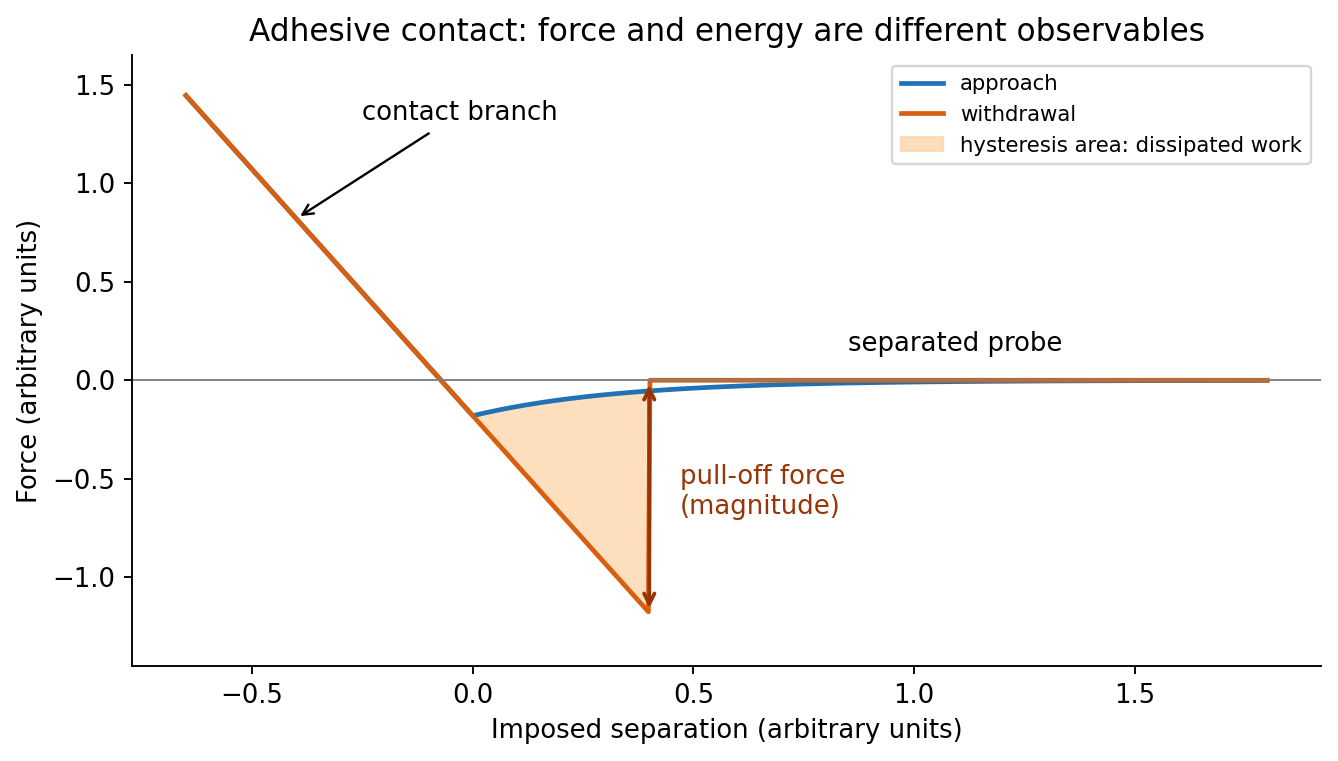
At position (1), the AFM probe is far from the surface, with approximately zero force. At (2), attractive interactions bend the AFM cantilever toward the surface; when the attractive force gradient exceeds the cantilever spring constant, the equilibrium becomes unstable and jump-to-contact occurs. Position (3) is on the mechanical-contact branch: changes in imposed height largely bend the AFM cantilever and, for a compliant specimen, indent the sample. This branch can include compressive contact and adhesive contact under tension; contact does not itself imply a positive force at every point. At (4), during withdrawal the tip remains attached and pulls the AFM cantilever downward until the pull-off force is reached and it detaches. Approach and retraction follow different paths because adhesion creates a hysteretic contact. The numbered points identify stages on the source curve, not four extra question parts.

piezoelectric scanner creep is the continued slow displacement after a step in scanner drive, even when the commanded voltage has stopped changing. The scanner's strain continues to relax, and the motion can resemble a slowly decaying, approximately logarithmic drift. After changing scan size, position or offset, early lines can therefore have stretched or compressed coordinates. Allow settling, avoid large abrupt moves, use a position-sensor closed-loop control system, and compare repeated images. This time-dependent response differs from the direction-dependent piezoelectric hysteresis and from ordinary thermal drift.

The repeated, similarly oriented rounded triangular outlines in panel (a) are characteristic of AFM tip convolution: a narrow raised object can image the shape of a blunt or contaminated AFM probe, rather than reveal its own lateral shape. A finite tip radius broadens lateral dimensions. Replace or clean the AFM probe, check it on an independently characterized sharp-feature standard, and repeat at low load; agreement after a tip change is stronger evidence than a visually pleasing image. Image processing cannot uniquely recover unmeasured sidewalls or prove that every particle with a similar outline is an artefact.

Panel (b) contains horizontal streaks associated with steep features. The natural instrumental diagnosis is AFM feedback artefact: the height controller does not track a rapid change faithfully, or rings after it. Reduce the scan speed and adjust proportional/integral gains below the oscillation threshold. Compare trace and retrace and rotate the fast-scan direction: a streak following the scan rather than the specimen is instrumental. Loose contamination can also produce scan-line streaks, so clean or change the AFM probe if tuning does not remove them. Tip-shape broadening in (a), and scan-direction tracking/streaking in (b), are the principal diagnoses; the images alone do not uniquely establish every underlying cause.

For $\omega \tau \ll 1$,andThus the material flows at sufficiently low frequency: its static shear modulus vanishes and its terminal response is viscous. The dashpot in the Maxwell branch allows its spring stress to relax, so there is no permanent elastic path through the parallel network.

The fact that both $G^{\prime }$ and $G^{\prime \prime }$ tend to zero is not evidence of a force-free material: stress at fixed shear rate tends to ${\eta }_0\dot{\gamma }$. At higher frequency the spring stores energy, but a finite-frequency elastic response does not make the long-time material a solid.

Let the Maxwell branch contain spring modulus $G$ and series viscosity ${\eta }_M$, in parallel with a dashpot of viscosity ${\eta }_s$. The branch strains are equal and stresses add. Writing ${\sigma }_M$ for the Maxwell stress,For $\gamma =\mathrm{Re}({\gamma }_0{e}^{i\omega t})$ and $\tau ={\eta }_M/G$,Multiplying the Maxwell fraction by $1-i\omega \tau$ givesThe sign of the imaginary coefficient depends on the phasor convention; these expressions use $e^{i\omega t}$, so $G^{\prime \prime }>0$ represents dissipation. In the time domain, the equivalent constitutive relation isThe original mechanical schematic shows the series spring/dashpot branch separately from the parallel dashpot.

A Kelvin-Voigt model element places a spring and dashpot in parallel, givingUnder a stress step from a relaxed state,It captures delayed but bounded material creep and eventual strain recovery after unloading, rather than steady terminal flow.

For an ideal strain step,After the loading impulse, the stress remains $G{\gamma }_0$. The model does not produce a gradual stress-relaxation tail at held strain. A real finite-rate ramp replaces the impulse by a finite dashpot stress during loading, but the subsequent held-strain stress is still constant. Thus this model describes material creep retardation but not a solid's genuine time-dependent relaxation toward another finite modulus.

A strain increment $\Delta {\gamma }_j$ applied at time $t_j$ contributesLinearity lets the contributions add, and time-translation invariance makes the kernel depend only on elapsed time:In the continuous limit this is Boltzmann superposition,The material's prehistory must be included, or it must start from a specified relaxed state. Aging, yielding and large-strain changes can violate this simple superposition. An instantaneous Newtonian contribution can be written separately as ${\eta }_s\dot{\gamma }(t)$; for an ideal step it is an impulse, not an ordinary finite relaxation tail.

In a material creep experiment, apply a small step shear stress ${\sigma }_{0}H(t)$ and measure the resulting strain. The creep compliance is $J(t)=\gamma (t)/{\sigma }_0$. An elastic solid reaches a bounded strain; a fluid can continue deforming.

In a stress-relaxation experiment, impose a small strain step ${\gamma }_{0}H(t)$ and measure stress while holding the deformation. The relaxation modulus is $G_{\mathrm{rel}}(t)=\sigma (t)/{\gamma }_0$ after the loading transient. A fluid's stored shear stress can decay to zero, while an elastic solid retains a nonzero long-time contribution.

The original curves distinguish the controlled input from measured output. The strain/stress must be small enough for linear response, and real finite loading rise time, instrument compliance, wall slip and temperature must be characterized. Otherwise an instrumental transient can be mistaken for a material relaxation mode.

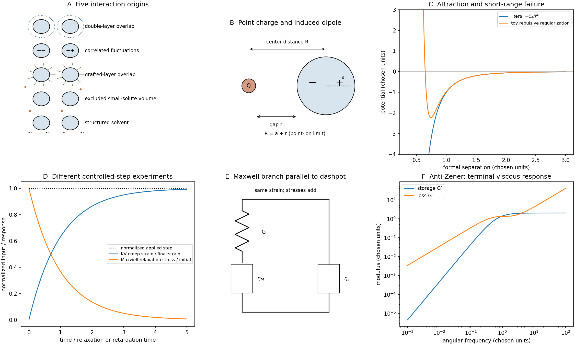
The literal $u(r)=-C_4/r^4$ curve is monotone increasing from $-\infty$ at $r\to 0^{+}$ toward zero from below as $r\to \infty$:Taken literally at a zero gap, it predicts an unbounded collapse energy and force. That extrapolation is outside the far-field dipole approximation and cannot describe actual touching matter.

Finite atomic/ionic dimensions, electronic overlap and Pauli repulsion supply short-distance constraints. Solvent and hydration layers, steric coatings and surface chemistry can add further contributions. An illustrative regularized model is $u_{\mathrm{toy}}=A/r^{12}-C_4/r^4$ with $A>0$; it has a finite minimum at $r=(3A/C_4{)}^{1/8}$ and becomes repulsive at shorter distances. This is a schematic regularization, not a derived complete ion–sphere contact law.

Separately, correcting the center-distance convention to $R=a+r$ already removes this particular $r=0$ divergence from the far-field expression, but does not make a dipole approximation accurate at contact. Near-field multipoles and microscopic repulsion still require a better model. Calibrated colloidal probe technique measurements can test where a long-range force model ceases to agree with actual approach curves.^[ref]

For $\alpha >0$, the given model predicts attraction proportional to $r^{-5}$ in force, independent of the ion's charge sign; the energy is proportional to $-r^{-4}$ and vanishes at large separation. A larger electric polarizability gives a stronger interaction.

This is induction by a charged object. Ordinary nonretarded London interaction between two small neutral polarizable objects instead has an $R^{-6}$ energy dependence; geometry-integrated colloidal dispersion laws can have other powers. Calling the specified $r^{-4}$ law a generic dispersion force would conceal its charge-dependent origin.

Attraction can favor association or adsorption. A stable suspension normally requires an opposing free-energy barrier, such as double-layer or steric repulsion, relative to Brownian motion. Salt, surface coatings and solvent quality alter that balance. However, one ion–particle pair potential alone does not establish the phase behavior or aggregation rate of a many-particle suspension; concentrations, diffusion, surface chemistry and the remaining interactions also matter.

Write $C_4=\alpha Q^2/[2(4\pi {ϵ}_0{ϵ}_r{)}^2]$. Differentiating the stipulated potential givesFor positive $\alpha$, the force points toward smaller separation for either sign of $Q$.

Its physical origin is charge-induced dipole attraction, rather than London dispersion forces. A point-charge field induces $\mathbf{p}=\alpha \mathbf{E}$ and the energy cost of inducing that moment gives $u=-\alpha E^2/2$. The charge changes the electric dipole moment; it does not, within this linear model, change the intrinsic coefficient $\alpha$. For a conducting sphere in a uniform medium, $\alpha =4\pi {ϵ}_0{ϵ}_r{a}^3$; other dielectric contrasts give another electric polarizability.

There is a distance inconsistency in the stated model: the point-charge field uses center-to-center separation $R$, whereas the question calls $r$ a surface gap. For a point ion and sphere, $R=a+r$. A controlled far-field dipole model therefore uses $u\simeq -C_4/(a+r{)}^4$, with $R\gg a$. The boxed derivative is the literal result for the given mathematical $u(r)$; it is not a justification for extending that dipole formula to contact.

A useful five-part classification is electrostatic double-layer, dispersion, steric, depletion force and solvent-mediated interactions. It is a practical classification rather than a unique exhaustive list.

Electrostatic double-layer forces arise from surface charge and mobile-ion redistribution. Like-charged surfaces often repel; opposite charges can attract. Their range changes with salt screening. London dispersion forces comes from correlated electronic fluctuations and is one contribution to Van der Waals force; its sign and strength across a medium depend on dielectric response.

steric stabilization occurs when adsorbed or grafted layers overlap, increasing chain confinement and/or local osmotic free energy. depletion force arises when smaller nonadsorbing solutes are excluded from a narrow gap: their greater accessible volume outside favors bringing the large particles together. Structured-solvent forces include short-range hydration force and hydrophobic attraction; their microscopic origin differs from the depletion force of an added solute.

The original sketches show double-layer overlap, a polymer-coated gap, depletion force exclusion and solvent structure, alongside a dispersion-potential curve. A realistic suspension can experience several simultaneously. Charge neutrality of a particle does not remove dispersion, steric or solvent-mediated interactions.