
At fixed temperature difference and constant internal resistance,Differentiation givesIt is positive below and negative above it, while power vanishes for an open or shorted load. Therefore the maximum power transfer theorem givesAt this point and half the electromotive force drops across the load. Maximum electrical power is not generally maximum thermal-conversion efficiency. If changing current also changes the temperature difference because the thermal source has finite impedance, the fixed- optimization must be reconsidered.
Use a Thévenin equivalent: an ideal voltage source in series with the internal resistance , driving the load .
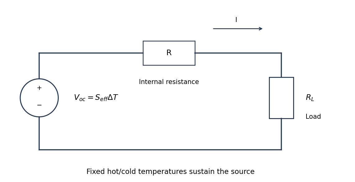
Original fixed-temperature-difference equivalent circuit of a thermoelectric generator, with internal and load resistances distinguished
. Details. The same current flows through both resistances, . The load terminal voltage is , smaller than the open-circuit voltage. The electrical battery symbol represents the maintained thermoelectric source under this model; heat input is still required.
A thermoelectric generator uses the Seebeck effect: a maintained temperature difference across suitable conductors produces an open-circuit electromotive force. For a pair of legs,when the effective Seebeck coefficient is approximately constant. Repeated p- and n-type legs are usually connected electrically in series and thermally in parallel.
Connecting a load lets part of the heat flowing from the hot side to the cold side become electrical power. Both a heat source and a cold-side heat-removal path are necessary: a uniformly warm device with no maintained temperature difference supplies no sustained output. Internal electrical resistance, heat leakage, contact losses and the finite temperature difference reduce the harvested power; the converter is a heat engine rather than a source of energy from temperature alone.
Interpret the stipulated model as a freely jointed chain with independent, isotropically oriented segments of length . With end-to-end vector , cross terms vanish on averaging:Using only the model's supplied segment size and count givesThe mean vector is zero, not the mean magnitude. In the three-dimensional large- Gaussian chain limit,Thus the common root-mean-square interpretation of an average chain size is , while the mean scalar distance is about . The contour length is a different quantity. A count of links between positions changes these estimates by less than .
These are results of the explicitly idealized statistical chain, not a prediction about the conformation or persistence length of an actual biological molecule. TODO (user-deferred biology): material-specific biological interpretation of that model.
For a polymer curve parameterized by contour distance , let be its unit tangent. The persistence length is the characteristic contour distance over which tangent orientations lose correlation. In the usual three-dimensional worm-like chain convention,where is the bending stiffness. Segments much shorter than look approximately straight; a much longer chain can contain many statistically distinct orientations.
A surface image can be traced to estimate tangent correlations as a function of contour separation, after accounting for tracing resolution and substrate effects. A strictly equilibrated two-dimensional chain has a different relation between bending stiffness and correlation decay length from the three-dimensional convention. The definition must therefore state whether the surface preserves a projected conformation or allows in-plane equilibration. This is a statement about statistical filament mechanics; biological interpretation is deferred.
Four useful interactions are dispersion attraction, electrostatic interaction, capillary attraction and short-range repulsion. Their ranges are relative to atomic contact and depend on geometry and environment.
Van der Waals forces provide an attractive contribution extending beyond direct atomic overlap; for an ideal sphere and plane it scales as in a simple nonretarded model. Electrostatic forces can also be long-ranged: biased conducting surfaces are commonly attractive, whereas charged insulating surfaces can attract or repel depending on their charge and screening.
A capillary meniscus in humid air can pull tip and sample together. It acts over the formation and rupture range of the liquid bridge and can greatly exceed atomically localized forces; it is not a universal interaction in a dry vacuum. At the shortest separations, overlap-related Pauli repulsion provides a steep repulsive contact contribution.
Atomic-scale contact contrast relies on strongly localized short-range tip–surface forces, especially the rapidly varying repulsive interaction in the simple contact-mode picture. Long-range attraction mainly adds a background. Real atomic-resolution imaging also depends on apex structure, stability and operating mode; a generic long-range force alone does not resolve individual surface atoms.
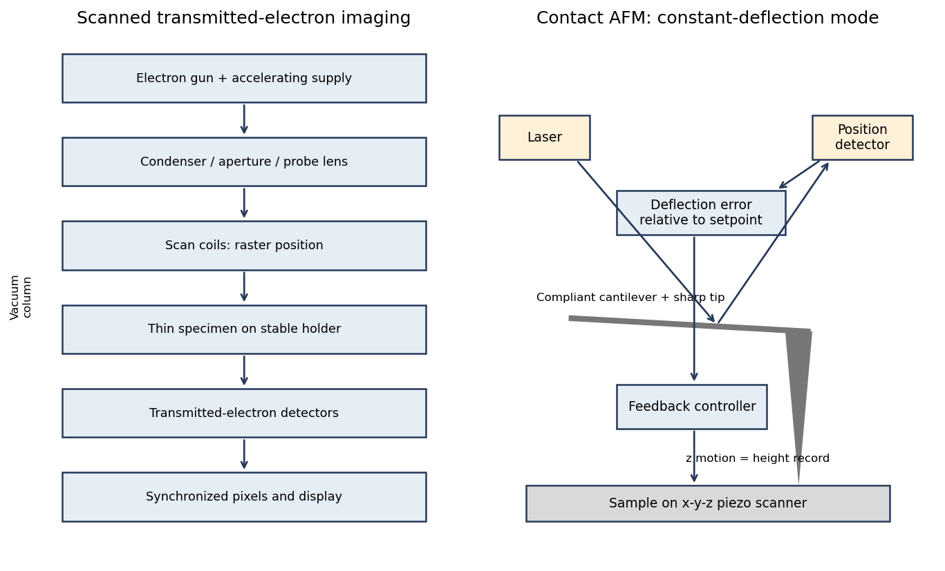
In contact-mode atomic force microscopy, a sharp tip on a compliant cantilever remains in contact with the surface while a feedback loop controls its normal deflection. A laser reflected from the cantilever onto a position-sensitive detector converts bending into an electrical error signal. With calibrated deflection and stiffness , the normal force is approximately under the stated contact convention.
A piezoelectric scanner raster-scans the sample or tip. The controller adjusts vertical position to maintain the chosen deflection setpoint; that vertical displacement is recorded as topography. The right panel of the microscopy diagram identifies tip, cantilever, optical deflection readout, controller and vertical actuator.


A real positive photoresist pattern usually has finite edge slope and rounding rather than mathematically sharp vertical steps. The optical aerial image and finite resist contrast give a graded exposure boundary. Absorption through the film, focus, reflections from silicon and development kinetics can make the opening narrower or wider at different heights.
Incomplete development can leave residual material at the floor; standing-wave exposure can cause sidewall ripples, and substrate-related chemistry can produce footing. Bake history and developer transport can modify corners and line width. An undercut can be engineered with a suitable resist stack, but it is not an automatic consequence of ordinary positive-tone processing. The final profile must therefore be measured rather than inferred solely from the mask artwork.
Let and be the open projected regions in the two layers. For normal, collimated rays, the transmitted opening is the intersectionAn upper particle blocks any lower-layer gap beneath its footprint. A translated layer can therefore reduce island size, suppress some islands or close the holes completely. If the projected openings coincide, an ideally registered second layer need not change the pattern at all. A rotated or differently registered layer can create a larger superperiod or a less regular pattern.
The additional height also increases the separation between some blocking edges and the substrate, making a finite angular source distribution more important. Deposition angle and layer separation then enter the projected aperture geometry. No unique double-layer pattern follows without specifying registry, orientation and source direction; the figure illustrates aligned and shifted possibilities instead of treating one as inevitable.
Treat the specified particles only as rigid geometric shadowing objects; no biological preparation or interpretation is needed. Their projected shapes are rounded-ended rods with straight central length and cap radius . Normal, collimated evaporation deposits metal in the gaps between projected particle footprints, leaving isolated small islands after mask removal, rather than a metal replica of each rod.
One concrete dense parallel packing has center translationsAdjacent rounded ends then touch at triangular arrangements. The open regions are small curvilinear triangular gaps near those ends. This is a specified geometrical packing for the sketch; the words close-packed do not uniquely prescribe the domain orientation or registry of all real sheets.
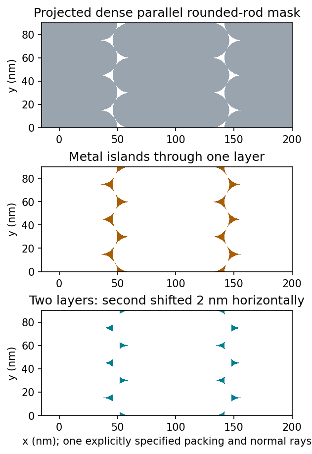
Original geometric calculation of rounded-rod shadow masks, deposited islands and the effect of shifting a second layer; no source illustration is reproduced
. Details. 
Particle size and shape distributions change the gap size and spacing. Misorientation, missing particles, boundaries between ordered domains, overlaps, incomplete coverage and drying-induced cracks interrupt long-range order. Substrate roughness and uneven adhesion distort the arrangement. A finite source angle produces deposition shadowing and penumbra; surface diffusion, island nucleation and increasing film thickness can broaden or merge deposited regions. These are generic geometry and materials effects, not assumptions about a biological assembly mechanism.
Flattening removes fitted components of the image whether they are instrumental or real. A true specimen slope, broad dome or slow height variation can be erased if it resembles the chosen background. Strong features can bias a fit and create false depressions, streaks or halos; an overly flexible polynomial can fit away scientifically useful topography.
Line-by-line correction can destroy real differences between terraces, especially when no common flat region spans the lines. Height statistics, roughness and feature depths then depend on masking and fit order. Report those choices and compare profiles before and after processing.
Flattening does not restore structures inaccessible to the tip, undo a double-tip artefact, remove finite-tip broadening, reconstruct a saturated signal or recover data lost to unstable feedback. It also does not calibrate the scanner. These limitations are important when a superficially smoother image is mistaken for a more accurate measurement.
Sample tilt and scanner bow are other common backgrounds that AFM image flattening can remove. Fit a plane to a genuinely flat reference area and subtract it to remove tilt. A low-order curved fit can approximate the vertical background produced by a piezoelectric scanner's non-planar motion.
Line-dependent offsets or slow drift can sometimes be removed by subtracting a reference level from each scan line. Mask pits, particles and true steps so that they do not bias the reference. An independently measured flat calibration specimen and scans in different orientations help distinguish instrumental background from actual specimen curvature.
AFM image flattening estimates an unwanted background and subtracts it from the recorded height:A plane removes overall tilt; a line-by-line constant or low-order fit removes line offsets or curvature. For a tip-change height jump, align the baselines of unchanged reference regions on either side of the event, using a piecewise offset or appropriately masked line fits. A single global plane cannot in general remove an abrupt step.
Exclude genuine features from the fit, use the same terrace as a reference where possible, and retain the unprocessed data. The corrected image has a consistent relative background; it does not establish that the interaction force, tip shape or absolute height calibration remained unchanged. In particular, flattening is a correction for the offset component of a tip-change artefact, not a repair of every consequence of a changed tip.
A tip-change artefact occurs when the effective apex changes during scanning, for example through material pickup, loss of an attached particle or damage. In tapping-mode atomic force microscopy, a sudden change can introduce a false height offset between parts of the image, even on a continuous terrace.
The change alters the probe–surface interaction or the effective point at which the chosen amplitude setpoint is reached. The controller moves the vertical scanner to recover that setpoint, recording a spurious step or a change in line baseline. The sign is not fixed: different apex changes can move the apparent surface up or down.
The amplitude channel usually shows a transient deviation as the interaction changes; with stable feedback it returns toward its setpoint. It therefore need not retain the same persistent offset as the recorded height. A change in probe resonance or free amplitude can also change the operating condition. If the apex geometry has changed, widths and shapes can change too, or duplicated structures can appear as a double-tip artefact. A baseline correction cannot recover these lost geometric data.
For a displayed width representing a scanned specimen width , the linear image magnification isThe user changes the scan-coil excursion, hence . A smaller raster displayed at the same width gives larger magnification. Changing the display or print size also changes displayed magnification, so the calibrated scale bar is more portable than a magnification label. This is the scan/display principle described in the manufacturer's microscope guide.[ref]
Scanning Electron Microscope A To Z by JEOL. Magnification of SEM, printed p.7: scan width and display width; the same raster-display geometry applies in STEM
At the low-magnification extreme, the probe scans the widest accessible field. Coil range, apertures, scan distortion and maintaining focus constrain the actual usable width. Formally increasing without bound would make arbitrarily small, but a real column has a finite accessible field.
At the high-magnification extreme, the scan covers a very small region. Formally makes diverge, but exactly zero scan width samples one location and supplies no spatial image. Electron microscope resolution, finite probe size, pixel spacing, drift, noise and specimen damage set the useful limit. Enlarging a field already sampled more finely than its resolvable information produces empty magnification, not new structural detail. For pixels across a field, the specimen sampling interval is ; this is distinct from the probe's spatial resolution.
There are unlisted articles, also show them or only show them.