
Work by Francis Rudolph Paolini 2026-10-18
Work by Francis Halzen 2026-10-18
Papain digestion of IgG 2026-10-18
Limited Papain digestion of IgG cuts each immunoglobulin heavy chain on the N-terminus side of the hinge crosslinks, releasing two Fab fragments and one Fc fragment.[ref]
The structure of a typical antibody molecule. Immunobiology: The Immune System in Health and Disease, 5th edition by Charles A. Janeway, Jr. and others; §3-3 and Figure 3.3: papain cut positions and two Fab plus one Fc
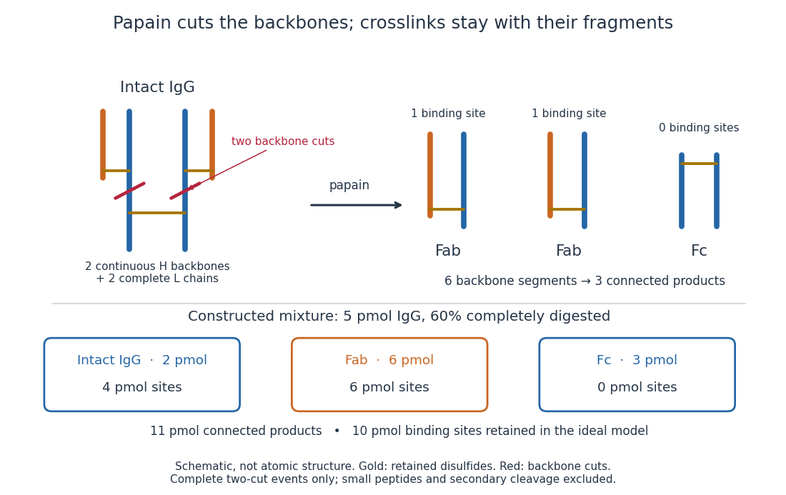
Two backbone cuts give two Fab fragments and one Fc fragment
. Original schematic of ideal limited Papain digestion of IgG, with cuts distinguished from retained protein disulfide bonds. The lower panel counts products for a constructed partial-digestion example, not a measured digest. Small released peptides, incomplete cleavage of one arm and secondary cleavage are excluded from that model. Details.
A connectivity argument explains the three products. Treat each continuous backbone segment as a graph vertex, and retained interchain disulfide bonds as edges. After the two stipulated cuts, six backbone segments remain: two complete immunoglobulin light chains, two immunoglobulin heavy chain arm segments and two immunoglobulin heavy chain stem segments. Each light chain remains attached to its own arm segment, producing two separate Fab fragments. The two stem segments remain attached to each other, producing one Fc fragment. Thus six backbone segments form three connected components of a graph, not six independently released products. Removing crosslinks instead, while keeping each backbone intact, would leave four chain components in this simplified covalent-connectivity model.
For a constructed mixture, start with of intact IgG and stipulate that undergoes the complete two-cut event while the rest remains intact. Count amount of substance of each product:The total amount of separately connected products becomes , although the starting amount was . Each digested IgG replaces one connected assembly with three. The antibody binding site inventory is conserved in this model:The factor two counts sites per intact IgG, not extra immunoglobulin light chains per Fab fragment. Fragment counts, backbone-segment counts and antibody binding site counts must be kept distinct. A real digest's retained binding would additionally depend on preservation of the paratopes.
The historical functional test was more subtle than asking whether a fragment still formed a visible precipitate. Rodney Robert Porter's earlier rabbit anti-ovalbumin preparation was digested with papain powder. The resulting fragment did not precipitate ovalbumin itself, but specifically inhibited ovalbumin precipitation with undigested antiserum. The intact-antiserum reaction supplied the positive comparison: failure to precipitate alone did not mean failure to recognize the antigen.[ref]
Separation and Isolation of Fractions of Rabbit Gamma-Globulin containing the Antibody and Antigenic Combining Sites by Rodney Robert Porter. Rodney R. Porter, Separation and Isolation of Fractions of Rabbit Gamma-Globulin containing the Antibody and Antigenic Combining Sites, 1958, opening paragraph: earlier papain-powder digest and inhibition of precipitation
The inference is that binding and assembly of a precipitating network are different abilities. A one-site Fab fragment can occupy an epitope without providing the two-arm bridge available to intact IgG. The inhibition readout supports retained recognition under the tested conditions; it does not locate individual contacts or show that every papain-generated product binds. This is the conceptual benefit of fragmenting an antibody: one can ask which functions survive loss of a structural connection.
Mass fractal dimension Created 2026-10-18 Updated 2026-10-24
The mass fractal dimension relates the particle count or mass in a self-similar aggregate to its spatial size. For primary particle radius and aggregate radius of gyration , a common convention is , with a nonuniversal prefactor . In three dimensions the mean occupied fraction scales as . A smaller therefore describes a more tenuous large cluster; a compact constant-density object has . The scaling applies between the primary-particle and aggregate scales, not at all distances.
Hermitian symmetry 2026-10-18
If is a real-valued function and an integrable function, its Fourier transform has Hermitian symmetry: . The value at negative frequency is the complex conjugate of the value at positive frequency.
Fourier transform of the hyperbolic secant 2026-10-18
For real , integrate around a rectangle of height . Its top-edge value is times the bottom-edge value, and the only enclosed simple pole is , with residue . The vertical-edge integrals vanish as their real parts tend to positive and negative infinity. The residue theorem gives , proving the stated Fourier transform identity. This is an example of a function reproducing its shape under a Fourier transform, up to rescaling.
Fourier transform of a truncated cosine 2026-10-18
For on and zero outside, the angular-frequency Fourier transform follows by writing the cosine as two complex exponentials. Combining fractions gives . The apparent singularities at are removable, with value . If , jumps at the endpoints give an oscillatory envelope. If , the function is continuous at the endpoints but its first derivative jumps, giving an envelope. This is an explicit instance of Fourier decay from a derivative jump.
Duality property of the Fourier transform 2026-10-18
For the Fourier transform convention , Fourier inversion at gives . Thus transforming twice reflects the argument and multiplies by . The identity holds directly on the Schwartz space, and extends to the L2 space and to tempered distributions. It lets an already known transform pair be used in reverse without another integration.
Fourier transform of a polynomial multiple 2026-10-18
With Fourier transform convention , differentiation under the integral gives , proving the displayed identity. For example it applies when all for are absolutely integrable, or in the tempered distribution sense. It is the dual counterpart of the Fourier transform of a derivative.
Inverse Fourier transform Created 2026-10-18 Updated 2026-10-24
With the Fourier transform convention , the inverse Fourier transform is the displayed linear operator. The integral is defined directly for an integrable function . The Fourier inversion theorem ensures under its hypotheses, in particular for Schwartz functions, and for integrable and at continuity points of . The operation also extends to tempered distributions; the normalization and sign depend on the chosen Fourier transform convention.
For , periodically extend and from with period . Their Fourier series areand, away from odd integers,The first identity follows by integration of on , using the antiderivativeFor the second identity, integration by parts and show that its sine coefficient is times the first series' cosine coefficient. This avoids assuming that a Fourier series can always be differentiated term by term. The periodic hyperbolic cosine is continuous, so its series converges to it everywhere. The periodic hyperbolic sine has a jump discontinuity at each odd integer: the Dirichlet-Jordan convergence theorem gives the average of its two limiting values, namely zero, there. Both identities hold in the sense of mean-square convergence, which suffices for Parseval's identity.
Translation of a Fourier series 2026-10-18
For a period- Fourier series written as , where , translating the function by to rotates each pair of Fourier coefficients:The constant coefficient is unchanged. These formulas follow by the sine and cosine subtraction identities. In the complex Fourier series, the same statement is . An integer-period translation changes no Fourier coefficient.
For , with period , half-wave rectification givesThe Fourier coefficients are , , , with all remaining coefficients zero. To derive the cosine coefficients, integrate over and use the product-to-sum identity. The sine coefficients follow from orthogonality. A half-period delay reverses only the fundamental sine term and leaves the constant and even-frequency cosine terms unchanged, by translation of a Fourier series.
Let and real . Extend with period . In the Fourier series convention , put . Direct integration givesFor example, the required antiderivatives are and . The Dirichlet-Jordan convergence theorem gives the exponential value away from the jumps and their midpoint at odd multiples of . For , the function is identically one, with and all other Fourier coefficients zero.
Let be nonzero real constants and let be a smooth periodic function of period , with real Fourier coefficients . Write the unknown periodic solution with Fourier coefficients . Fourier orthogonality applied to the equation givesSolving these two-by-two linear systems givesThe smooth forcing has rapidly decreasing Fourier coefficients, so the resulting series and its derivatives converge and satisfy the equation. Uniqueness follows because the difference of two solutions is , which is periodic only when . A single sinusoidal forcing therefore gives a single sinusoidal response with changed amplitude and phase.
Fourier series of a noninteger-frequency cosine Created 2026-10-18 Updated 2026-10-20
Extend from with period . It is an even function, so all sine Fourier coefficients vanish. The product-to-sum identity givesIndeed, integrate on and use . ThusThe coefficients are , so the series converges absolutely and uniformly. The Dirichlet-Jordan convergence theorem identifies it with the periodic function everywhere, including the endpoints because the two endpoint values agree. Substituting a noninteger rational frequency and a convenient yields explicit series sums. Integer frequencies require taking removable limits rather than substituting into a zero denominator.
Wiener-Khinchin theorem Created 2026-10-18 Updated 2026-11-05
For a complex weakly stationary process with finite second moment and continuous uncentered autocorrelation , there is a unique finite positive spectral measure of a stationary random field. With the optical sign convention, write it asThe sign reverses the frequency coordinate relative to the alternative positive-exponential convention. To see the positivity behind the theorem, expand . This makes the correlation a positive-definite function, so Bochner's theorem supplies the measure.[ref]
245C, Notes 2: The Fourier transform by Terence Tao. Bochner theorem immediately before Exercise58; applied here to the positive-definite correlation function
An ordinary power spectral density exists when . If is integrable, . Stationarity alone does not guarantee such a density. For at every time and , the correlation is one and .
The normalized Lorentzian line shape gives . Its width therefore describes decay of temporal coherence. A persistent spectral line instead contributes an atom, which cannot be treated as an ordinary integrable density.
Cross-correlation Created 2026-10-18 Updated 2026-10-20
For this sign convention, cross-correlation compares a function with translated copies of another, conjugating the first factor. If , Fubini's theorem gives Fourier transform . Indeed, the substitution factors the double integral into and . The zero-lag value for is the squared L2 norm. Fourier inversion applied to this correlation proves the Parseval identity, first for Schwartz functions and then by density for L2 space.
Four-wavevector Created 2026-10-18 Updated 2026-10-24
The four-wavevector combines the angular frequency and spatial wavevector of a plane wave. Phase invariance gives . Under a boost , , and . For metric signature , is a Lorentz scalar. A vacuum light wave has .
Three-momentum Created 2026-10-18 Updated 2026-10-20
Three-momentum is the spatial part of a particle's four-momentum, . Its components depend on the reference frame, while is a Lorentz invariant.
There are unlisted articles, also show them or only show them.