
Eddy-damped quasi-normal Markovian closure 2026-10-14
EDQNM closure models the evolution of the turbulent energy spectrum through spectral triad interactions. Fourth-order correlations are approximated using products of second-order correlations, an eddy damping limits the resulting triple correlations, and their memory integrals are replaced by expressions using current spectra. The modeled damping times are additional physical input. This allows evolving spectra and scale-dependent transfer, but does not automatically recover coherent structures or internal intermittency. Bertoglio, Squires and Ferziger's simulation comparison explains the damping assumptions and tests their limitations.
Constant-skewness turbulence closure 2026-10-14
This turbulence closure assumes the velocity increment skewness is the same throughout the equilibrium range, with its value fixed by the Kolmogorov two-thirds law and Kolmogorov four-fifths law. It yields a simple crossover between differentiable and inertial-scale increments, but suppresses the scale dependence of skewness and has no independent spectral-transfer dynamics.
A trigonometric polynomial of degree at most obeys the displayed derivative bound. Iteration gives . Applied to differences of approximants at dyadic degrees, this inequality underlies the inverse theorem for trigonometric approximation. It differs from the endpoint-weighted Bernstein inequality for algebraic polynomials.
Tridiagonal solve costs 2026-10-14
For the displayed unpivoted Thomas algorithm with one right-hand side, count each scalar addition, subtraction, multiplication or division as one arithmetic operation. Forming takes five arithmetic operations per forward step. The last unknown takes one division; each remaining back substitution step takes three arithmetic operations. ThusThis is an operation-count model, excluding assignments, indexing, pivot checks and any special simplifications of the coefficients. It is not a timing benchmark. The original tridiagonal matrix needs scalar entries, and its right-hand side another . Overwriting with and with , then with , keeps storage ; the arrays, rather than the few loop temporaries, determine the total space complexity.
For repeated right-hand sides, retain the LU decomposition: computing once costs arithmetic operations, and each subsequent pair of forward substitution and back substitution sweeps costs . Hence right-hand sides cost arithmetic operations. This is the banded counterpart of Reusing LU factors for multiple right-hand sides.
An invertible matrix need not admit the unpivoted Thomas algorithm. For example,Here and , but makes undefined. Interchanging the two equations instead gives the upper triangular matrix system , , solved immediately by back substitution. Even a nonzero first diagonal does not guarantee all later pivot elements: has determinant , yet .
For a general tridiagonal matrix, use a solver with partial pivoting when these structural guarantees are unavailable or a dangerously small pivot element occurs. Adjacent row interchanges can introduce a second upper diagonal, so a pivoted solver must track that additional fill-in; it cannot blindly continue the unpivoted recurrence relations. LAPACK's
DGTSV explicitly performs partial pivoting, stores this extra upper diagonal, and includes it in back substitution. Its fixed-width storage and bounded work per row retain time for one right-hand side and storage.[ref]DGTSV (LAPACK 3.12.1) by LAPACK project. DGTSV, Purpose lines 34–39; DL argument lines 63–69; adjacent interchange lines 188–199; back solve lines 295–305
Safe pivots for tridiagonal elimination 2026-10-14
The displayed Thomas algorithm requires every modified pivot element to be nonzero in exact arithmetic. Nonzero original diagonal entries alone are insufficient: later pivot elements can vanish after elimination. Two useful sufficient contexts are a real symmetric positive-definite matrix, and strict diagonal dominance by rows:For the symmetric positive-definite matrix case, elimination leaves positive-definite remaining blocks by the Schur complement, so each . Equivalently, the initial principal minors are positive, and with .
For strict diagonal dominance, a short induction shows . The first row gives . Assuming the preceding bound, the triangle inequality givesIn particular . These are structural guarantees against a zero pivot element, not universal bounds on forward error in floating-point arithmetic. A poorly conditioned linear system can still amplify roundoff error; numerical stability and the condition number must be distinguished.
Consider the original small Poisson equation exampleIts exact solution is the quadratic polynomial . Use a uniform mesh with and three interior unknowns . The finite difference method replaces the negative second derivative byMultiplying by and moving the prescribed Dirichlet boundary conditions to the right givesThe endpoint values contribute and to the first and last equations; they are not additional unknowns. The Thomas algorithm givesand back substitution yieldsAll three values equal exactly: the centered finite difference for the second derivative is exact on a quadratic polynomial. This special nodal exactness does not assert exactness for arbitrary forcing or for the piecewise-linear curve joining the nodes.
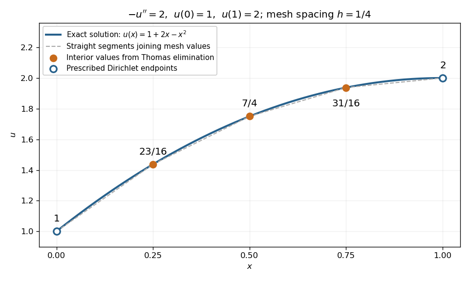
Exact quadratic Dirichlet Poisson solution and the three interior values recovered by tridiagonal elimination
. Details. For any interior points with , the scaled tridiagonal matrix has and . Its pivot elements are : start at and use . All are positive. Interior rows have equality in diagonal dominance, so strict diagonal dominance is not the reason this example works. Instead it is a symmetric positive-definite matrix, since for a real vector with ,Zero would force every neighbouring value equal and hence all values zero. This connects the boundary constraints directly to the safe pivots for tridiagonal elimination.
Tridiagonal elimination recurrences 2026-10-14
Let . Store the tridiagonal matrix by its diagonal , lower diagonal , and upper diagonal . The linear system iswith the nonexistent endpoint terms omitted. Initialize and . For , compute the elimination multiplier, modified pivot element, and modified right-hand side:These recurrence relations apply the elementary row operation after the preceding row has already been reduced. The transformed linear system is an upper bidiagonal matrix:Thus back substitution is especially short:For , only remains. Check each pivot element before its first division, including before back substitution.
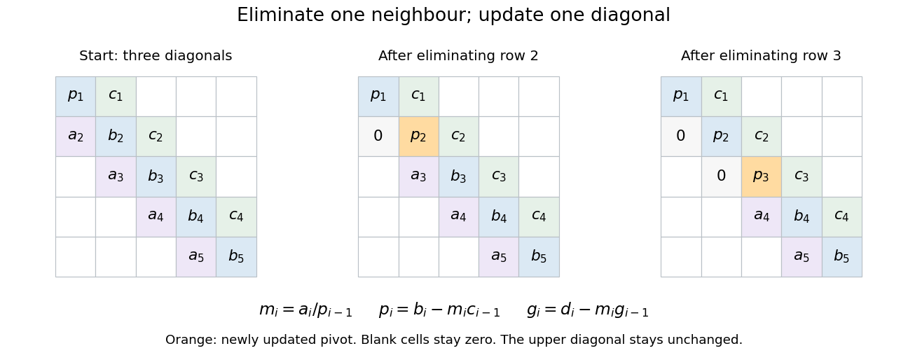
Tridiagonal elimination preserves the narrow band: only one row and one diagonal coefficient change per step
. Details. Equivalently, this constructs an LU decomposition with unit lower bidiagonal matrix , whose lower diagonal is , and upper bidiagonal matrix , whose diagonal is and upper diagonal is . The sweep is forward substitution in . There is no fill-in outside these bands when no rows are interchanged. LAPACK's
DGTSV source uses these same coefficient and right-hand-side updates in its branch without row interchange.[ref] Square triangular number 2026-10-14
A square triangular number is simultaneously a triangular number and a perfect square. For example, . This differs from a squared triangular number: is not itself triangular, by the recognition criterion for triangular numbers. Writing gives , a Pell equation that explains why this intersection of two counting patterns has additional arithmetic structure.
Squared triangular number 2026-10-14
A squared triangular number is the square of a number , where is a triangular number. Beginning at , the values are . Nicomachus's theorem gives them a second description as cumulative sums of cubes of numbers.
Recognition criterion for triangular numbers 2026-10-14
A nonnegative integer is a triangular number exactly when is a perfect square. Its square root is then an odd integer, and the row index isCompleting the square in proves necessity; reversing the calculation proves sufficiency. For example, , giving . In contrast, lies strictly between and , so twenty is not a triangular number. The criterion turns an apparently open-ended search through a sequence into one exact perfect square check.
Triangular number square-complement identity 2026-10-14
For ,An -by- array of cells has cells. One side of the diagonal, including the diagonal itself, contains cells; the other contains . For , the two counts are fifteen and ten, giving twenty-five. The identity is stated in Introduction to Arithmetic by Nicomachus (Hahn teacher edition) (Book II, Chapter 12, §§1–2, printed p. 70).
Triangular number pair-counting identity 2026-10-14
For distinct objects, the number of unordered pairs of different objects isOrdering the objects gives pairs with the first object, new pairs with the second, and so on down to one. Alternatively, ordered pairs count every unordered pair twice. The binomial coefficient therefore counts the edges of a complete graph on vertices. This is also consistent with the handshaking lemma: each vertex has degree of a vertex , and the degree sum counts every edge twice.
Triangular number recurrence 2026-10-14
For a positive integer , adding the row of length to the previous arrangement gives . Thus the first differences of the triangular numbers are . The triangular number recurrence provides incremental computation: after , adding seven gives .
Circumcircle 2026-10-14
The circumcircle of a nondegenerate triangle is the unique circle through its three vertices. Its center is the circumcenter, found by intersecting two perpendicular bisectors; equality of distances to all three vertices proves existence, and subtracting the squared-distance equations proves uniqueness. For a right triangle, the midpoint of its hypotenuse is equidistant from all vertices, so its circumradius is half the hypotenuse length.
Incircle of a triangle 2026-10-14
The incircle of a triangle is the circle inside the triangle tangent to all three sides. Its center is the intersection of two internal angle bisectors; its radius is , where is the area and the semiperimeter. To prove it is the largest contained circle, let any candidate have center , radius and distances from the three side lines. Splitting the triangle into three triangles with vertex gives . The tangent circle attains equality, proving maximality. For a right triangle with legs and hypotenuse , , since and .
Similar triangle Created 2026-10-14 Updated 2026-10-20
Two triangles are similar if a Euclidean similarity maps one onto the other. Their corresponding angles agree, and corresponding side lengths have a common positive ratio.
Specify the correspondence first: matches , matches and matches . For similar triangles, the common scale factor satisfiesThe ratios compare matching sides in the same order. A Euclidean similarity can also move, turn or reflect the triangle; its orientation on the page is irrelevant. In the Euclidean plane, matching just two interior angles is enough: their sums force the third to match, and equal corresponding angles force the side ratios to agree. This is the angle-angle (AA) criterion for similar triangles. Matching just one angle is insufficient.
Scale the right triangle with vertices , and by . Its new vertices are , and , and its side lengths are . The matching side ratios are . Both triangles have a right angle and the same two other interior angles, approximately and . However, their areas are and : doubling lengths multiplies area by four.
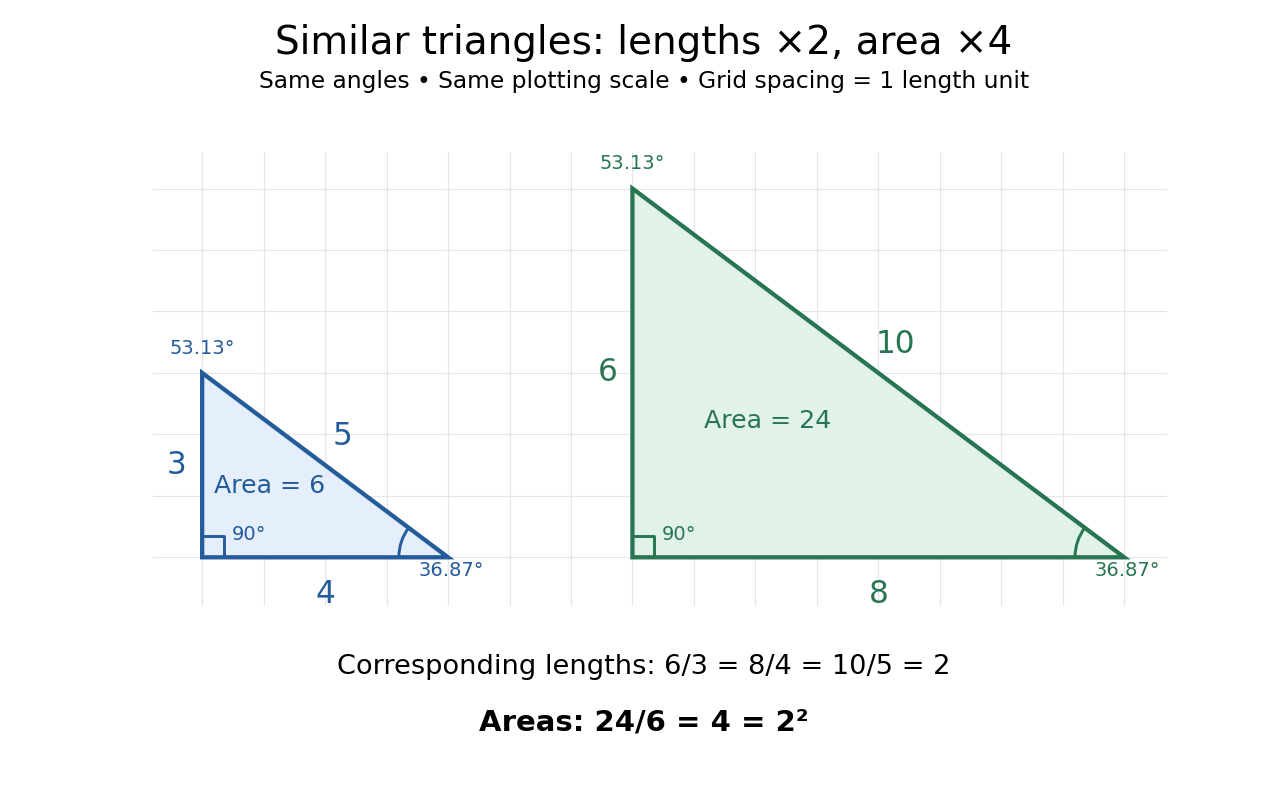


Generally, a Euclidean similarity multiplies both a base and its perpendicular height by , so the area becomes . This explains why an enlarged drawing needs four times as much surface when each length doubles. It also enables indirect measurement: under assumptions of level ground, vertical objects and parallel light rays, an object of height casting a shadow of length provides a right triangle. Another object's shadow of length gives a similar triangle and height . The shared angles justify the inference; visual resemblance alone does not.
Euclid's Elements VI, Definition 1 describes similarity using corresponding angles and proportional sides. VI.4 establishes the implication from matching angles to matching side ratios, while VI.19 states the squared relation between side ratios and areas. These are documented ancient formulations of the principles used above, without establishing a first discoverer.[ref][ref][ref]
https://mathcs.clarku.edu/~djoyce/elements/bookVI/propVI19.html. Euclid, Elements VI.19
Marginally outer trapped surface 2026-10-14
A closed spacelike two-surface is marginally outer trapped when its future outgoing null expansion is zero. For the future black-hole type, the ingoing null expansion is negative. An apparent horizon on a chosen spatial slice is ordinarily its outermost such surface under suitable regularity assumptions. The notion depends on the slice and is not the global definition of an event horizon.
TE wave equation in a stratified magnetodielectric Created 2026-10-14 Updated 2026-11-05
With permittivity and permeability depending only on and time dependence , a transverse electric polarization obeys the displayed equation. Maxwell's equations give and . The latter satisfies . At normal incidence ; the nonzero magnetic component is .
Hamiltonian transport equation 2026-10-14
Transport along a Hamiltonian flow. The solution is wherever the inverse characteristic exists. Equality of mixed derivatives makes the transport vector field divergence-free, so its flow preserves phase-space volume. Smoothness of the Hamiltonian alone gives local characteristics, not a complete flow on all of phase space.
There are unlisted articles, also show them or only show them.