
Work by Walter Bradford Cannon 2026-10-14
Skin friction coefficient Created 2026-10-14 Updated 2026-11-05
The local skin friction coefficient normalizes wall shear stress by the outer dynamic pressure:For the ideal Blasius boundary layer on one face of length , averaging the local skin friction coefficient gives . The factor of two follows from integrating , not from counting both plate faces. Drag on two equally exposed faces doubles when the reference area remains that of one face.
Trail in a graph 2026-10-14
A trail is a walk whose edge sequence has no repetitions. Its vertices may repeat, including its first and last vertices. The zero-length walk is a trail because it repeats no edge. Every graph path is a trail, but the converse fails: the trail in the shared example isIts six edges are pairwise distinct, although occurs twice. Visiting a junction again and traversing a road segment again are different events.[ref]
https://people.math.binghamton.edu/zaslav/Oldcourses/581.S99/notes.html. Thomas Zaslavsky, Supplementary Notes for Graduate Graph Theory: trails and paths
In an undirected graph, traversing and then repeats the same edge; direction of travel does not give it a new identity. In a multigraph with distinct parallel edges joining and , the closed walk is a trail, whereas is not. Both have the same vertex sequence . In a directed graph, separate directed edges and may instead be used once each; record their identities and obey their directions. Thus testing a trail means checking the actual edge records, not merely checking consecutive endpoint labels.
For a finite graph, a trail has length at most ; unrestricted walks can have arbitrarily large length whenever a positive-length closed walk exists, since it can be repeated. An Eulerian trail is the special trail that uses every edge, so its length is exactly . Our length-six trail omits and is therefore not an Eulerian trail. In a road-inspection model, a trail describes servicing its selected segments once while allowing returns to junctions; requiring service of every segment leads to the Eulerian trail question. If extra travel between serviced segments is necessary, the complete journey can be a walk even when each segment is serviced only once. This distinction keeps the service requirement separate from the route actually travelled.
Finite mean matters in Wald's equation 2026-10-14
For a simple symmetric random walk starting at zero, let be its first hitting time of . The infinite mean first passage of a simple symmetric random walk shows that almost surely but . Since , assuming a finite expected value for would let Wald's equation assert , a contradiction. The formal expression is not an allowed use of the theorem.[ref]
Compare . From every surviving position in , three consecutive positive increments force absorption within three steps. Each fresh block has probability of this event, so and . This establishes finiteness before invoking the theorem. If is the average remaining time from position , the law of total expectation givesso . Symmetry gives equal exit probabilities at and , and , as Wald's equation predicts. This is a small gambler's ruin problem with two absorbing barriers.
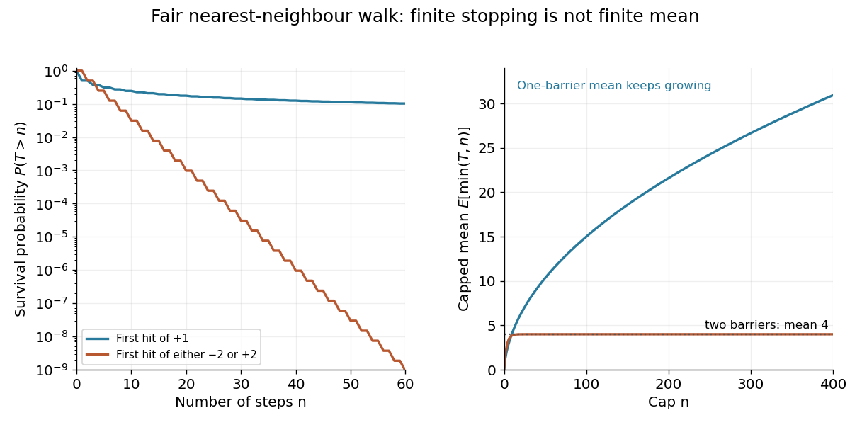

Even for , each bounded stopping time satisfies . The stopped process tends to almost surely, but its expected value does not tend to . Rare long negative excursions retain the balancing contribution. The existing stopped-walk martingale with almost sure but not L1 convergence explains the related failure of uniform integrability; almost sure convergence alone does not permit exchanging a limit and an expected value.
Peeking ahead in a random sum 2026-10-14
Let be independent fair signs, each taking and with equal probability. Set if , and if . Deciding whether requires the second sign, so is not a stopping time for the natural filtration. The four equally likely possibilities giveBoth the increments and the count are bounded, but the identity fails because the second contribution is retained only when it is negative. This is selection using an unobserved outcome, rather than a legitimate sequential decision. Boundedness alone cannot replace the stopping time hypothesis.[ref]
Cost of trials until the first success 2026-10-14
Consider a stipulated repeated-attempt model, with independent Bernoulli trials of success probability . An unsuccessful attempt costs three units of work, and a successful attempt costs one. Let be its success indicator function, its cost, and the first success. Observing reveals , so is a stopping time for the costs' natural filtration. The geometric distribution gives and , including the deterministic case . ThusAt , the average is four attempts and ten units of work. An independent check uses the pathwise identity : there are failures and one final success. No success probabilities or costs in this example are measured data.
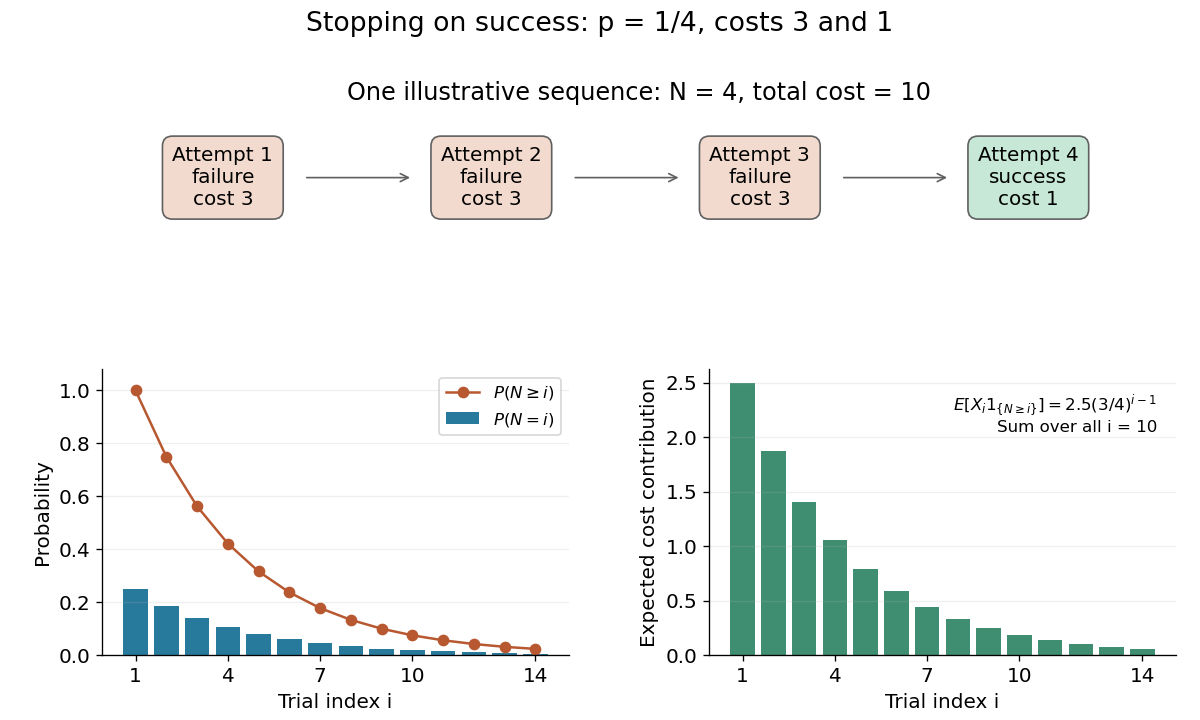
Cost and survival probabilities for stopping at the first success
. Original stipulated model with success probability , failure cost three, and success cost one. The top shows one illustrative stopped sequence; the lower panels show exact probabilities and the contributions to the expected value from each admitted step. Details.
Here is not independent of the observed costs. In particular, conditioning on forces every preceding cost to be three and the final cost to be one, so , generally different from at . Nevertheless the unconditional identity holds. This distinction explains why conditioning on the total count as though the original cost law remained unchanged is a faulty proof.
Line vortex Created 2026-10-14 Updated 2026-11-05
An ideal straight line vortex in a two-dimensional incompressible flow has circulation and induces velocityIts stream function, with , is . Positive means counterclockwise circulation. In an ideal point-vortex description, the vortex position is advected by the regular velocity produced by the other vortices and the boundaries; its own singular velocity is excluded.
Vortex dynamics 2026-10-14
The evolution of a vorticity distribution together with the velocity field it induces. A transport equation advances vorticity; diagnostic inversion recovers velocity from it and the specified boundary conditions.
Entropy of an orthogonal quantum mixture Created 2026-10-14 Updated 2026-11-05
For density operators supported on mutually orthogonal subspaces, the eigenvalues of their mixture are , where are the eigenvalues of . Substitution into the definition of Von Neumann entropy gives the displayed decomposition into Shannon entropy of the label and the mean entropy within each block. Zero eigenvalues use .
Entropy continuity from Jordan decomposition Created 2026-10-14 Updated 2026-11-05
For density operators in dimension , let . The positive and negative parts of their difference have the same trace . Normalize them as and write . Applying the two entropy bounds for a quantum mixture to this common state proves the displayed bound. The function is increasing and concave, with , which also controls average entropy errors in pure-source compression.
Vaughan's identity 2026-10-14
For thresholds , write and similarly for the other truncations. Vaughan's identity isIt decomposes a sum weighted by into short, Type I, and Type II bilinear sums.
Specific volume 2026-10-14
The volume per unit mass; for a uniform substance it is the reciprocal of mass density. The Clapeyron equation pairs a difference of specific volumes with latent heat per unit mass.
Volume per particle 2026-10-14
The volume divided by the positive number of particles . The Van der Waals equation uses this convention for , whereas specific volume divides by mass and molar volume divides by the amount of substance. With the Avogadro constant , the molar volume is .
Molar volume 2026-10-14
The volume per amount of substance, with measured in moles. For a uniform pure substance, , where is its molar mass and its mass density. The Clapeyron equation pairs a difference of molar volumes with latent heat per mole.
Spherical volume conductor model 2026-10-14
A spherical volume conductor model approximates a conducting body by a sphere, usually with uniform or radially stratified conductivity. It provides explicit forward models for electroencephalography and magnetoencephalography. Its symmetry makes a radial current dipole magnetically silent outside the sphere; departures from spherical symmetry need not retain that property.
Geselowitz formula 2026-10-14
For a homogeneous volume conductor with an insulating boundary , the Geselowitz formula expresses the exterior magnetic field as the primary Biot-Savart law field minus a surface contribution from the induced electric potential. For a current dipole, . On a spherical boundary, is parallel to , so the surface term has zero radial component at the observation point.
Volterra iteration for a singular power-series problem Created 2026-10-14 Updated 2026-10-25
The iteration , successively appends terms of the displayed series. Induction verifies the iterates, and factorial denominator bounds give convergence with derivatives on compact sets. Its limit is the power series solution of , , .
Planar viscous-sheet stretching equations 2026-10-14
A symmetric thin viscous sheet with shear-free faces has leading longitudinal velocity independent of thickness coordinate , and incompressibility gives . Young–Laplace equation and the Newtonian fluid stress tensor give and . The effective longitudinal tension per unit transverse width is . The last two terms include the horizontal projections of the two surface tension pulls. Force balance gives , yielding the displayed longitudinal equation; the face kinematic conditions give the displayed conservation of mass equation.
Convex viscous potential minimum principle 2026-10-14
An inertialess fluid flow with symmetric stress generated by a convex viscous dissipation potential minimizes among fields satisfying the prescribed velocities, and any incompressibility constraint. The supporting-hyperplane inequality bounds the difference of two functional values below by . Integration by parts, equilibrium and on the velocity boundary make this lower bound zero. A pressure reaction has zero contraction with divergence-free variations. Convexity proves global minimality without asserting uniqueness.
Prandtl limit Created 2026-10-14 Updated 2026-10-25
The Prandtl limit observes a high-Reynolds number flow within a shrinking wall-normal layer. For streamwise distance and outer speed , rescale the normal distance by and the normal velocity by . Convection and normal viscous diffusion then remain comparable, while streamwise viscous diffusion is smaller. The leading normal momentum equation makes pressure independent of the rescaled normal coordinate, and the tangential equation is the Prandtl boundary-layer equation. This laminar asymptotic balance is local and need not remain valid through separation or instability.
There are unlisted articles, also show them or only show them.