
Symmetric Hermite integral obstruction 2026-10-14
Suppose nonzero algebraic numbers form a Galois-stable set, with Galois-invariant integer weights , and is an integer. Choose vanishing at all with , and a positive integer making all algebraic integers. For a large prime , put and , and let be the sum of its derivatives. The weighted sum is an integer, nonzero modulo when . If the displayed exponential expression vanished, integrating along the finitely many segments to would bound that nonzero integer by . This contradiction proves the obstruction and supplies direct proofs for and .
Schneider-Lang theorem 2026-10-14
Let be meromorphic functions with for a fixed number field . Suppose are algebraically independent over and have finite orders . The set of points where every is finite and belongs to satisfies the displayed bound. The orders are growth orders for meromorphic functions. For , , the orders are zero and one and the functions are algebraically independent; an algebraic value of at nonzero algebraic would produce infinitely many such points .
Steady-state tracking error 2026-10-14
The steady-state tracking error iswhen this finite limit exists. A finite steady-state tracking error does not require the reference signal, the plant output, or the control input to become constant: all can grow while their difference settles. If the tracking error grows without bound or keeps oscillating, report that behavior rather than assigning a finite steady-state tracking error. Eventual accuracy and asymptotic stability are different questions.
For the first-order low-pass filter introduced in reference signal, assume exact measurement, constant control disturbance , and no actuator saturation or feedback delay. Under proportional control with , a constant reference signal givesThe decaying homogeneous solution has rate , so this equilibrium point is approached from any finite initial condition. A nonzero tracking error is needed to maintain the control input that balances the model's tendency to relax toward . This differs from the accumulating controlled plant , for which proportional control already tracks a constant reference signal exactly when . The presence or absence of a step offset depends on both the controlled plant and the controller.
For a ramp reference signal , the same proportional control givesIts long-time particular solution grows with slope when . Thus the controlled plant and homogeneous closed-loop response are stable, but the tracking error has no finite steady-state tracking error. A changing goal requires a different performance test from a fixed destination.
Now use proportional-integral control , , with . For the same controlled plant, differentiate the error equation on intervals where the inputs are smooth:The characteristic polynomial has both roots of a polynomial in the open left half-plane: real roots have negative sum and positive product, and a nonreal complex conjugate pair has negative real part. This proves decay of the homogeneous error for this model. It does not prove stability of an arbitrary controlled plant controlled by positive gains. At a reference jump, use the original ordinary differential equations to set the new initial conditions, rather than treating the reference as smooth at that jump.
With a constant reference signal and constant control disturbance, proportional-integral control therefore gives . At its equilibrium point, , , and . The stored integral maintains the required command while the current tracking error vanishes. For a ramp reference signal, however, the forcing above is , andThe tracking error settles even though the accumulated integral and the required control input grow. This finite offset is the error needed to keep increasing that command. For with , the forcing is and even this proportional-integral control leaves a tracking error growing with slope . Integral action is therefore a precise mechanism for selected input classes, not a promise of perfect tracking for every reference signal. [ref]
https://www.fbswiki.org/wiki/index.php/PID_Control. Åström and Murray, Feedback Systems, Chapter 11: integral action and actuator limits
Here are completely explicit synthetic examples with , , and no sensor bias. Choose , per percentage point, percentage point per degree, and percentage points per degree-second. Thus is dimensionless, and . In the following formulas, denotes the numerical time in seconds and denote numerical temperature rises in degrees. For the unit-step reference signal , proportional control and proportional-integral control respectively giveFor the ramp reference signal , the corresponding solutions areThe control inputs here are numerical heater-command percentage points. Substitution into and into the controller equations checks these solutions without invoking an unverified limiting rule. The proportional control step offset is degrees; the proportional-integral control step offset is zero. The proportional control ramp error grows; the proportional-integral control ramp offset is degrees, exactly .
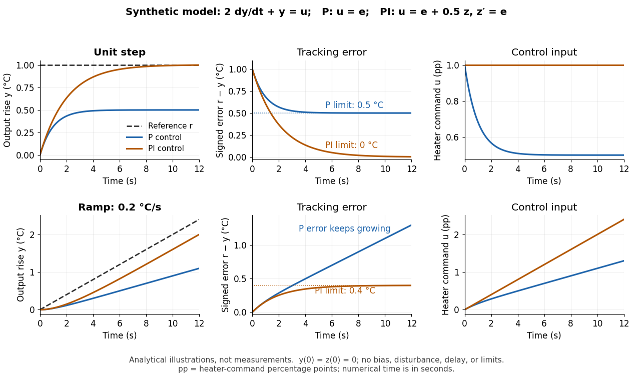
Synthetic step and ramp tracking of one stable first-order low-pass filter
. Original analytical model curves, not measurements or fits to the temperature laboratory. Columns compare plant output with reference signal, signed tracking error, and control input; rows use a unit step and a ramp of degrees per second. Both designs have decaying homogeneous responses. Proportional-integral control removes the step offset but leaves the ramp offset degrees; proportional control has an increasing ramp error. Heater-command percentage points and output degrees use separate axes. Details.
The conclusions have specific limits. With constant sensor bias , stable proportional-integral control for a feasible constant reference signal drives the measured tracking error to zero but leaves the physical discrepancy . Under proportional control, the measured offset instead becomes . If actuator saturation prevents the required control input, zero step offset is not achievable by these formulas. A changing control disturbance contributes to the error equation, while feedback delay can change stability; neither is covered by the constant-disturbance result. These restrictions are what make steady-state tracking error useful: it identifies the input, measurement convention, and model for which an accuracy claim is actually justified.
Pure-target upper bound on trace distance 2026-10-14
For two normalized pure states, the difference of their projectors has two eigenvalues , giving that trace distance. Write a mixed density operator as . Convexity of the trace norm and weighted Cauchy-Schwarz inequality give . Thus a small probability of failing the pure-state projector test forces trace-distance proximity, including for correlated multipartite outputs.
Trace distance for qubit dephasing 2026-10-14
For the pure qubit , subtracting the output of dephasing channel leaves a Hermitian matrix with zero diagonal and off-diagonal modulus . Its two eigenvalues are that number and its negative, giving the displayed trace distance. For real , this is .
By the variational characterization of trace distance, maximize over . The adjoint of a quantum channel is positive and unital, so . Moving the channel onto therefore restricts, rather than enlarges, the effects available in the input variational problem. This proves the displayed bound for every pair of density operators.
Trace distance between qubit states 2026-10-14
For qubit density operators, the trace distance has a particularly simple geometry. Write their Bloch vectors as in the Bloch ball:where is the identity operator and denotes the Pauli matrices. This Bloch vector representation includes both pure states on the Bloch sphere and mixed states in the interior of the Bloch ball. [ref]
The Pauli matrix multiplication law gives . Hence the two eigenvalues of are , and their absolute sum givesThe trace distance is half the straight-line Euclidean distance between the Bloch vectors, not the angular or surface distance along the Bloch sphere. Opposite Bloch vectors have trace distance one; the centre is at trace distance from every pure state.
For the pure states and , the Bloch vectors are and . Their straight-line separation is , soThese Bloch vectors are perpendicular, but the pure states are not orthogonal: . The Helstrom measurement for the zero and plus states measures along the difference direction , rather than along either input Bloch vector.
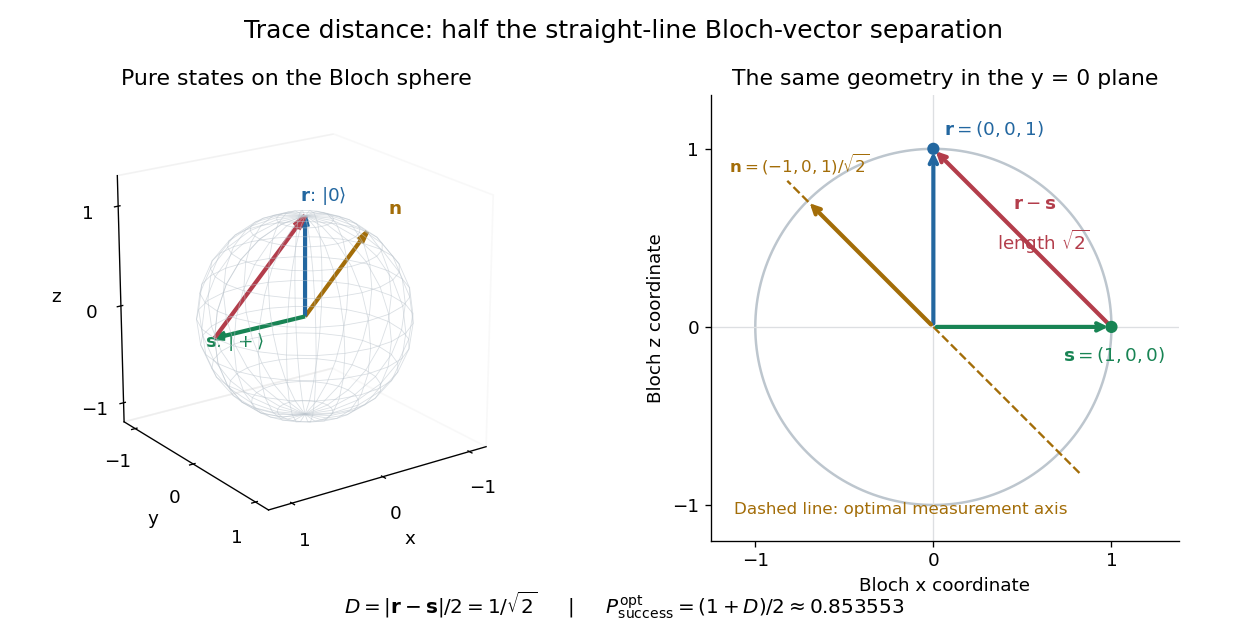
Trace distance is half a Bloch-vector chord, and the optimal zero-versus-plus measurement follows the difference direction
. Details. 
Finite-horizon total progeny generating function Created 2026-10-14 Updated 2026-10-25
Count the ancestor and the next generations of a Galton-Watson process. Conditioning on the ancestor's offspring, their independent descendant trees each have the preceding finite-horizon probability generating function, proving the displayed recursion. If the count instead excludes the ancestor, the recursion is with . The indexing convention must be specified.
Historical source for total correlation 2026-10-14
The abstract of Information Theoretical Analysis of Multivariate Correlation by Satosi Watanabe (1960, printed p. 66) names the sum of individual information entropies minus joint entropy "total correlation." It presents this as the finest grouping of the variables and identifies applications to geometric pattern recognition and shuffling cards marked zero or one. The name therefore connects the uncertainty of a system with the structure linking its parts; the worked integer parity and noisy-integer parity models here are separate examples calculated from their stated laws.
Scope and scale of total correlation 2026-10-14
For finite alphabets, , soFor identical copies of one fair bit, the upper bound is attained and total correlation is bits. Adding another copy increases the result without introducing a new underlying random choice. The choice of coordinates and their grouping therefore matters when comparing systems of different sizes.
For more general random variables, the relative entropy against the product of the marginals supplies a definition of total correlation that may be infinite. Subtracting differential entropies is justified only when those quantities are finite and the entropy identity is valid; an undefined difference of infinities is not a definition. The finite-alphabet examples above avoid that problem entirely.
Relative entropy to a product law 2026-10-14
Let be a joint probability distribution on a finite product alphabet, with marginals . Compare it with a product model , assuming wherever . Adding and subtracting the logarithm of givesThe first term is the unavoidable error from discarding dependence; the other terms are errors in the individual marginal probability distributions. Averaging a term that depends only on under is the same as averaging it under , which proves the identity directly.
Among product laws, the choice minimizes this relative entropy, leaving exactly total correlation. The related cross-entropy equals entropy plus relative entropy identity interprets this as extra average logarithmic loss from using the independent model. It is a statement about a specified joint law and loss function, not a claim that fitting a finite sample automatically recovers that law.
Chain decomposition of total correlation 2026-10-14
For finite alphabets, expanding joint entropy with the chain rule for information entropy givesEach term is mutual information with an entire preceding block, rather than necessarily with one preceding variable. Changing the order changes these individual terms but leaves their sum unchanged.
For the noiseless parity constraint and total correlation, and bit. The conditional block term supplies exactly the dependence that the pairwise comparisons missed. For three identical copies of a fair bit, the two block terms are both one bit. Thus total correlation counts total departure from the product law, not merely the presence of a single irreducible multiway relation.
Parity constraint and total correlation 2026-10-14
Let be independent fair bits and set , their exclusive or. The four possible triples are , each with probability . Every coordinate is fair, and every pair has all four outcomes with equal probability. Thus each pair's mutual information is zero, as in pairwise independence does not imply joint independence.
The full random vector has joint entropy bits, while the marginal information entropies sum to three bits. ConsequentlyThe product of the marginals predicts probability for every triple, including the four impossible ones. On each possible triple, the ratio of true to product probability is ; averaging its base-two logarithm gives the same one bit of relative entropy.
The example gives a concrete use for joint information measures. A lossless source coding scheme that treats the three coordinates separately needs three bits here. If the decoder knows the integer parity rule, the encoder can send just and let the decoder reconstruct exactly. Pairwise independence does not reveal that saving. This is a stipulated source law and an explicit two-bit code, rather than a promise that arbitrary data can be shortened.
Use , , positive pressureless matter and positive cosmological constant, with and no radiation. The Friedmann equation gives . Set , then . The remaining integral is , proving the formula by the beta function integral. Its two endpoints converge for positive densities, but the lifetime diverges in either pure-fluid limit.
Damped torsional oscillation 2026-10-14
A damped torsional oscillation is rotation about a fiber's fixed reference orientation with a restoring torque and dissipative torque. In the ideal viscous model, damping contributes with constant . This is a rotational damped harmonic oscillator. For known constant moment of inertia and torsion constant , define . In the oscillatory regime , and are set by the initial state. Successive positive peaks measured from the same equilibrium have magnitudes and ; their ratio gives . Consequently a measured damped oscillation period and decay together recoverUsing only underestimates the torsion constant in this model. The toy curve in torsion constant sets , , and . It gives , , and . Ignoring the decay recovers , an underestimate; including it recovers the stipulated torsion constant.
These equations assume a single rotational mode, a stationary zero, linear elasticity, and viscous damping. Internal fiber losses need not behave as a constant viscous coefficient: Fleischer and colleagues model their precision apparatus using a loss angle. Their response is evidence for specifying a damping model, not for applying the viscous correction universally. [ref]
Toric scheme over a base ring 2026-10-14
Given a dual pair of free lattices and a rational fan, glue over common-face charts. The monoid rings are semigroup algebras. A lattice map respecting cones gives a toric morphism. This construction works over a commutative ring , including , and also for an infinite fan in toric geometry.
// Target: toric-geometry.bigb
Lattice in toric geometry 2026-10-14
First Tor of a cyclic quotient Created 2026-10-14 Updated 2026-11-05
Let be a ring, a right ideal, and a left module. Then and the resolving modules in this argument are right -modules, while the second tensor factor is a left -module. Start a free resolution of with and a free module surjecting onto . The next differential presents the relations in . Right exactness of the tensor product of modules identifies with . Taking degree-one homology then gives the displayed kernel formula. Hence vanishing for every ideal is equivalent to the flatness criterion using ideals.
Tor for a principal non-zero-divisor quotient Created 2026-10-14 Updated 2026-11-05
For a commutative ring and a non-zero-divisor , resolve by . Tensoring with gives the kernel and cokernel in the displayed formula; all higher Tor functors vanish. Resolving either argument gives the same homology by the two filtrations of the double complex of the two free resolutions. For , both degrees zero and one equal .
Continuous linear operator Created 2026-10-14 Updated 2026-11-05
A continuous linear operator is a linear map that is continuous for the topologies of its domain and codomain. Between normed vector spaces, continuity is equivalent to an operator bound for some finite , so the terms bounded linear operator and continuous linear operator coincide there.
For general topological vector spaces, sending every bounded set in a topological vector space to a bounded set is a weaker property. For example, the identity from the weak topology on an infinite-dimensional Hilbert space to its norm topology maps bounded sets to bounded sets by the Uniform boundedness principle, but is not continuous. A basic weak zero neighbourhood only restricts finitely many linear functionals, leaving a nonzero common-kernel direction with arbitrarily large norm.
Thus the operator norm interpretation of boundedness used throughout numerical linear algebra belongs to the normed-space setting. In other vector topologies, specify continuity explicitly.
There are unlisted articles, also show them or only show them.