
Past exam of the mathematics course of the University of Cambridge 2004 iii Paper 79 1 Solution Created 2026-10-03 Updated 2026-10-14
Choose depth positive downwards and harmonic time dependence . At normal incidence, P waves and the two polarizations of S waves are independent scalar problems: a P wave uses the longitudinal modulus , and an S wave uses the shear modulus . In a uniform layer with wave speed and seismic impedance , write velocity and compressive traction asAt a perfectly bonded interface the velocity and traction are continuous. For incident velocity wave amplitude one from medium 1 into medium 2, these two conditions are and . ThusReflection is determined by seismic impedance, not by speed alone. A step to larger seismic impedance reverses the reflected velocity/displacement field waveform; the pressure reflection coefficient has the opposite sign. Its transmitted pressure coefficient is . Equal seismic impedance eliminates the reflection even when speed and wavelength change. At a free surface traction vanishes and velocity reflects with coefficient ; at a rigid surface velocity reflects with coefficient .
The mean elastic-wave energy flux is for positive real . Therefore the reflected and transmitted energy fractions areA displacement field transmission coefficient greater than one is compatible with conservation of energy; its flux must be weighted by the receiving seismic impedance.
For many layers, use the seismic layer transfer matrix. A layer of thickness has wave phase thickness andThis follows either by eliminating between the two faces or by integrating and . For the complete stack put . With upper and lower half-space impedances , an outgoing lower wave satisfies . Solving this condition gives the input seismic impedanceHere is lower-face velocity divided by upper-face incident velocity, including the propagation wave phase. For lossless layers and real frequency, . This supplies a sensitive check on any spreadsheet or numerical implementation; it is not correct simply to multiply the individual interface transmissions and discard the elastic waves.
The physical reason is repeated wave interference. In one layer between media 0 and 2, let denote the velocity coefficients above and . The first transmitted wave has wave amplitude . Every extra round trip supplies . Summing the geometric series givesIn the time domain the successive arrivals are delayed by , producing reverberation. In the frequency domain the same delayed terms produce resonant maxima and minima. For a layer between identical half-spaces of impedance ,At the layer transmits all the incident energy: the internally elastic waves cancel the direct reflection. Halfway between these resonances, a large impedance contrast gives strong reflection. For unequal exterior impedances, a quarter-wave layer with transforms its lower load to , again giving zero reflection at its design frequency. This matching is narrow-band.
Periodic alternation produces a periodic seismic multilayer stop band. For a cell of two layers with total thickness , the cell matrix has reciprocal eigenvalues , soWhen the absolute value of this expression exceeds one, the infinite periodic medium has no propagating cell mode; a long finite stack has exponentially small transmission. The energy is reflected, not absorbed. Pass bands instead contain oscillatory transmission peaks, becoming more numerous as the stack length increases. Disorder removes the exact cell periodicity but not multiple scattering or frequency-selective interference.
For a concrete reproducible investigation, take , equal one-way travel times in both layer types, exterior impedance , and frequency coordinate . At each layer is a quarter wavelength; one cell has diagonal matrix entries . For cells,It is about for one cell, for four cells and for eight cells. The infinite-cell stop band is . The accompanying calculation also shows the first transmitted arrivals for a single high-impedance slab: their wave amplitudes are at times . Their sum is one, consistent with unit zero-frequency transmission. These calculations illustrate both the spectrum and the pulse train without assuming access to the course's spreadsheet.
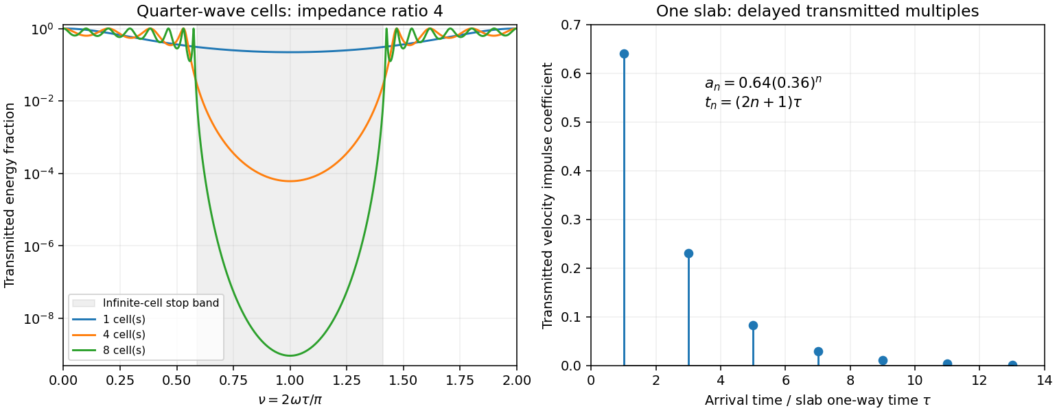
Original transfer-matrix calculations showing a periodic stack stop band and the transmitted reverberation train of one slab
. Details. Finally, as for a fixed finite stack, every , so the response approaches that of a direct interface between the exterior half-spaces. Equal exterior impedances give . For wavelengths much longer than a repeating cell, expansion of to first order instead gives an effective medium with averaged mass density and harmonic-mean modulus , where . Its speed is , not generally the arithmetic mean of the layer speeds. Attenuation makes the energy balance an inequality, while for a fixed oblique horizontal slowness the scalar SH calculation uses and . Oblique P-SV waves require coupled displacement field and traction matrices because of mode conversion at a planar elastic interface. Thick evanescent layers require scattering or impedance recursion rather than exponentially ill-conditioned transfer-matrix products.
Past exam of the mathematics course of the University of Cambridge 2004 iii Paper 78 3 Solution Created 2026-10-03 Updated 2026-10-14
For a linear viscoelastic fluid, causal superposition givesThe relaxation modulus is the stress response to a unit small step of shear strain. The equation assumes an isotropic reference state and deformations and rotations small enough over the significant memory times that nonlinear transport and strain products can be neglected. Small-amplitude motion can have high frequency; linearity does not require low frequency by itself. The infinite-past integral encodes the preceding history, rather than assuming that stress vanishes whenever the present rate vanishes.
For a small constant shear rate maintained from the remote past, the rate can be taken outside the integral. Therefore the zero-shear viscosity isprovided the kernel is integrable, with any instantaneous contribution counted fully. A nondecaying solid-like modulus would not yield a finite fluid viscosity.
To linearize the stated Oldroyd-B model, put and absorb the isotropic into pressure. The products of the small deformation tensor C and velocity gradient are second order. Using the paper's derivative-index-first gradient convention therefore givesAn integrating factor, with the prescribed preceding history, gives . Thus the linear nonpressure stress isThe regular relaxation tail is , while the solvent is instantaneous. Equivalently, the instantaneous solvent term in a relaxation modulus can be represented byHere the causal endpoint delta is defined by . If instead a symmetric Dirac delta is assigned half its mass at the endpoint, the same solvent term is written . Stating the convention prevents a factor-of-two error in the viscosity; the explicit stress formula above has no such ambiguity.
In a cone-and-plate rheometer, the small-angle gap is and the local wall speed is , so the shear rate is independent of radius to leading order: . Write for shear stress and for its polymer part. The linear constitutive response isThe uniform shear stress gives torqueFor the initial steady torque T, put and , . The steady polymer stress is , with . Hence the initial angular velocity is
For , the total stress is , but the polymer stress is continuous at the torque reversal. Since , a finite jump in shear rate is possible even though P cannot jump. Its immediate value isEliminating P from the constant-stress equations for givesThe decay time is the Retardation time of an Oldroyd fluid . Solving this first-order equation with the actual initial value yields the complete torque reversal of a linear Oldroyd fluid:In particular, but is more negative. The stored polymer stress initially retains its old positive sign, requiring a larger negative solvent shear stress to attain the new negative total torque. This produces the backward-speed overshoot and its subsequent relaxation. Apparatus inertia would smooth the instantaneous jump, but is neglected in the question. The torque must be sufficiently small for the entire transient, including its enhanced initial rate, to remain in the linear viscoelastic regime; small pre-reversal rate alone is not sufficient when is large.
Past exam of the mathematics course of the University of Cambridge 2004 iii Paper 78 2 Solution Created 2026-10-03 Updated 2026-10-14
A generalized Newtonian fluid can approximate the shear response of a fluid with viscoelasticity when the flow varies slowly relative to its stress-memory time scales and elastic stresses are negligible, or in locally steady unidirectional flow where a fitted steady shear viscosity captures the relevant stress and elastic normal stresses do not significantly influence the motion. It is not a general replacement in rapidly changing flows or in flows controlled by elastic stresses. Two specific failures are stress relaxation after deformation stops, since this law has no memory, and nonzero normal-stress differences in steady simple shear flow, since the only nonzero nonpressure components are off diagonal. A rate-dependent viscosity alone cannot repair either limitation.
Take the usual physical power-law fluid range , , and . The steady unidirectional Couette-Poiseuille flow satisfies . The stated upper-wall stress thus givesPut . Inverting this monotone stress law gives . Integration from the lower no-slip boundary condition gives the power-law Couette-Poiseuille flow profileThe upper no-slip boundary condition requiresThe bracket is a strictly increasing function of with value zero at , so the equation determines a unique positive . The absolute values are essential: for sufficiently strong pressure driving, the shear can reverse inside the channel. For a Newtonian fluid, , , and the bracket reduces to , yieldingFor zero pressure gradient the limit is pure Couette flow; the parameterization of wall stress by then becomes singular rather than indicating zero Couette stress.
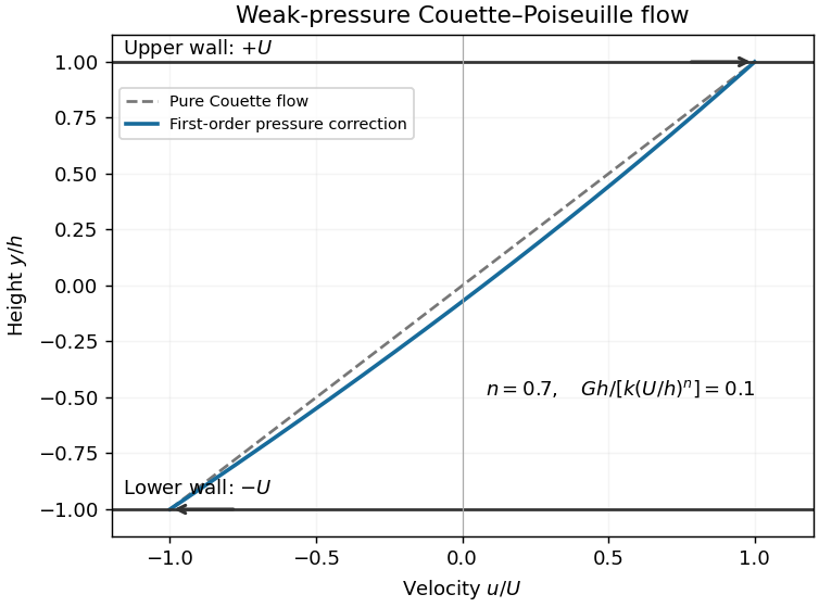
For weak pressure forcing, let and . Write the center-plane shear stress as . Linearization of the power-law relation about the positive base shear givesIntegrating across the channel must still give . The Gy term has zero mean, so at first order. Hence the weak-pressure Couette-Poiseuille expansion isIt is a small positive parabolic displacement of the straight Couette profile, preserving both wall velocities. For fixed positive n the stated controls the expansion; when n is very small one needs the stronger incremental condition .


The volume flux per unit spanwise width is . The odd Couette part contributes zero and the parabola contributes times its coefficient, soThis correctly reduces to the exact Newtonian flux at .
The extension to a general smooth generalized Newtonian fluid uses its differential shear viscosity, rather than its secant viscosity. Let for positive shear rate, and assumeLinearizing the stress law repeats the preceding calculation with replaced by . ThusThe expansion requires small rate changes, , and a smooth constitutive law on the perturbed rates. At zero differential viscosity the regular first-order expansion fails. A negative differential viscosity is still locally invertible mathematically, so the formula is formally applicable, but belongs to a decreasing, mechanically unstable constitutive branch. The usual stable-flow interpretation requires positive differential viscosity. Thus “any” generalized-Newtonian law needs these local qualifications.
Past exam of the mathematics course of the University of Cambridge 2004 iii Paper 78 1 Solution Created 2026-10-03 Updated 2026-10-14
Let two observers be related by , with Q a proper rotation matrix. A spatial second-rank tensor has material frame indifference if its values at corresponding events satisfy . This defines an objective second-rank tensor, and allows the observer's rotation to depend on time.
For Cauchy stress tensor, consider a material surface element with unit normal n and contact traction . A rigid observer change preserves its area and rotates both its normal and actual contact force: , . Thus for every n, proving . Fictitious body forces of an accelerated observer do not alter this transformation of physical contact traction.
To keep the vorticity convention explicit, write , and , the negative of the usual component-first spin tensor. Equivalently, with the derivative-index-first used in the paper, . Put , which is antisymmetric. The transformed velocity is , and direct differentiation givesThe additional observer spin cancels from the symmetric part, proving that the rate-of-strain tensor is objective.
Along the same material particle, differentiating givesThe two extra terms cancel those from . Moreover . Hence the complete objective time derivative satisfiesThis proves covariance for every constant scalar ; changing the spin convention without changing the commutator sign would not. It is a Gordon--Schowalter derivative with the paper's slip-parameter convention.
For the Johnson-Segalman fluid, first use the standard uniaxial extensional flow , with . Here and E is diagonal. The steady conformation equation giveswith vanishing off-diagonal components on the stable steady branch. The tensile normal-stress difference is . Dividing by the extension rate gives the Johnson-Segalman extensional response:The conformation tensor evolution in each principal direction is . Therefore a positive, attracting steady conformation requires both displayed denominators positive. For the first pole is at ; for it is at in the transverse components. At a pole the corresponding component grows linearly in time, and beyond it generically grows exponentially. The model has a finite-rate extensional catastrophe; the algebraic viscosity cannot be continued as a physical steady response past the first pole. At zero rate, , giving Trouton ratio three. For the polymer contribution to stress disappears and the response is simply Newtonian.
The question does not specify extension geometry. If a planar convention is intended instead, the same diagonal calculation gives , valid on the stable branch . The preceding boxed formula uses the standard uniaxial definition of extensional viscosity.
For simple shear flow , write , , , and . The xx, yy and xy components of the steady constitutive equation giveSubstituting the first two relations into the third yields , with . Define the viscometric functions by , and , using x for flow, y for the shear gradient and z for vorticity. The Johnson-Segalman steady viscometric functions are thereforeThe solvent creates no normal-stress differences in this flow. For nonzero , the fluid is shear thinning with positive first and negative second normal-stress differences.
To classify the stress curves, set and . The scaled shear stress is , andThe second term has minimum at . Thus the shear stress is monotone for and has a decreasing segment for . At equality it has a horizontal tangent but no decreasing interval. Below the threshold, its maximum and minimum occur atwith the smaller root giving the maximum. Negative-rate curves are obtained by odd reflection.
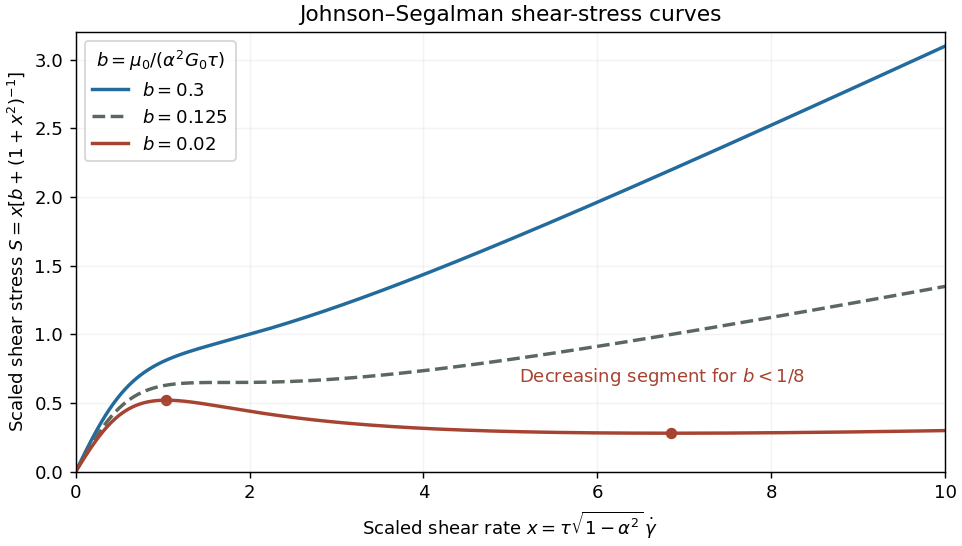
Monotone, marginal and nonmonotone Johnson-Segalman shear-stress curves
. Details. 
For small b, polymer stress dominates the low-rate response, while the solvent restores a positive high-rate slope. The Johnson-Segalman negative-slope shear threshold signals a constitutive instability of homogeneous shear: different local shear rates can carry the same shear stress, permitting shear banding. A stress plateau or a selected interface position cannot be inferred from the local curve alone; spatial regularization and boundary/history information matter. This limitation is illustrated in a primary diffusive Johnson-Segalman study. If , the scaling by b is inapplicable and the stress is just .
There are unlisted articles, also show them or only show them.