
Past exam of the mathematics course of the University of Cambridge 2004 iii Paper 73 3 Solution Created 2026-10-03 Updated 2026-10-14
The hydrostatic buoyancy anomaly is , and its leading adiabatic evolution is . The small vertical velocity advects the background stratification; vertical advection of the perturbation buoyancy is higher order. ConsequentlyThe impermeability condition at a stationary lower boundary is . Using gives the topographic buoyancy boundary condition for quasi-geostrophic flowFor application at the reference plane, the actual small-height condition is . Slopes scaled by are of Rossby-number order, so this topographic contribution is retained alongside the small ageostrophic vertical velocity. The dimensional slope should not be compared to the Rossby number without also specifying the aspect ratio.
The basic quasi-geostrophic streamfunction is . It gives , basic buoyancy gradient , and spatially constant interior quasi-geostrophic potential vorticity. Linearizing its conservation law therefore givesThe printed equation omits the shear-advection term. This cannot be omitted for general disturbances: an interior anomaly proportional to is materially conserved but not independent of time at a fixed location. The intended zero-interior-PV Eady model modes do have and satisfy both expressions; the ensuing mode calculation is valid in that subspace.
At either boundary, linearizing the geostrophic material derivative includes . LetThe two boundary equations areThese are exactly the respective bottom and top slope corrections to the rigid-boundary buoyancy condition for quasi-geostrophic waves.
Assume periodicity horizontally and first consider . Multiply its defining equation by and integrate over the layer. The two horizontal Laplacian terms vanish by integration by parts; the remaining volume term after one vertical integration is an -derivative. ThereforeFor nonzero , the boundary equations giveThe top advection term integrates to zero. Subtracting proves conservation of the boundary pseudomomentum of a sloping Eady layer:The original PDF uses squared vertical derivatives and the upper slope in the first denominator; these details are corrupted in the converted TeX. For arbitrary nonzero interior PV the same calculation instead gives , which need not vanish. For example, at an instant take , independent of ; the zonal average of is . Thus the boundary-only conservation statement also needs the zero-interior-PV qualification.
For an exponentially growing smooth normal mode, this qualification is automatic: the interior equation is , and a phase speed with nonzero imaginary part cannot equal the real basic velocity. Therefore . If , the conserved boundary quadratic form is definite, so a nonzero exponentially growing boundary amplitude is impossible. Instability consequently requiresfor . When one vanishes, the corresponding boundary derivative is simply advected and must vanish for a growing mode. The other boundary then yields a real single-edge-wave speed; if both vanish, the zero-interior-PV Neumann problem has no nonzero growing mode. These degenerate cases are neutral and should not be handled by dividing by zero.
For equal slopes, put , , , and . The normal-mode interior equation is for the zero-interior-PV modes. ThusThe coefficient equations areSetting their determinant to zero, without dividing by or , givesso the Eady model with parallel sloping boundaries hasFor positive , is the printed , and is the printed . The expression is even in the sign of that vertical scale. For the radicand is at least , so both speeds are real and these modes have no exponential growth. For equal slopes the earlier necessary condition is merely , which is satisfied in many stable cases and is not sufficient. At the speeds are and ; the invariant with nonzero denominators cannot be used, but the determinant still correctly gives neutral modes. No claim excluding transient amplification is needed.
Past exam of the mathematics course of the University of Cambridge 2004 iii Paper 73 2 Solution Created 2026-10-03 Updated 2026-10-14
Let , , and define the quasi-geostrophic streamfunction by . Use horizontal scale , vertical scale , velocity scale and advective time . The required quasi-geostrophic approximation has small Rossby number , , and Burger number . Hydrostatic, thin-layer scaling has ; density variations are small compared with , as required by the Boussinesq approximation. The leading horizontal flow is nondivergent, with vertical velocity . Retain forcing of the same slow order as density advection, ; stronger forcing need not preserve this balanced scaling.
Leading geostrophic balance and the hydrostatic approximation giveWrite . The density equation becomesTaking the curl of the horizontal momentum equations at the next order and using continuity gives the stretching equationSubstitute the expression for . Vertical differentiation commutes with the geostrophic material derivative acting on here: the extra Jacobian is . Since depends only on height, this yields the diabatically forced quasi-geostrophic potential vorticity equationThe minus sign is appropriate to the specified density forcing; a positive upward buoyancy forcing is and gives .
Now take constant and linearize about rest. Put and . The forced equation isFor the harmonic heating response of quasi-geostrophic flow, represent the two traveling Fourier components with frequencies and :Each component of the forcing has amplitude , soEquivalently its vertical structure obeysThese are the time-periodic forced responses; unspecified initial data may add free Rossby waves. Selecting no incoming waves describes forcing switched on causally and then its persistent harmonic part.
For , the eastward component always has . Let . The growing exponential would introduce an unbounded velocity and pressure disturbance at infinity, so discard it. The bottom condition then givesIf , this expression has the regular limit , rather than a physical singularity.
For , the westward component also has positive . Choose and use the same decaying expression with minus subscripts, including the same coincident-exponent limit. Thus both components are vertically evanescent above the heating.
For , putBoth homogeneous solutions are bounded, so boundedness is insufficient. A free Rossby wave with phase hasThe radiation condition demands energy propagation away from the heating, upward into . For that selects positive , hence in the westward component. The resulting solution isIt satisfies and, away from the decaying forcing, . Its far-field amplitude does not decay in this nondissipative model: continuous forcing supplies an outgoing wave train. Thus the low-frequency westward component propagates vertically while the eastward component remains evanescent.
At the threshold , the westward vertical wavenumber is zero. Excluding the linearly growing homogeneous solution and retaining the bottom condition gives . This bounded limiting response tends to a constant and has zero vertical group velocity; demanding both bottom zero and decay to zero at infinity would overdetermine this threshold problem. For , the branch labels and propagation inequality must be reconsidered; the comparison stated here assumes the usual positive beta-plane gradient.
Past exam of the mathematics course of the University of Cambridge 2004 iii Paper 73 1 Solution Created 2026-10-03 Updated 2026-10-14
Write and , with . For the profiles below take , so agrees with the stated parameter; changing the sign of reverses the balanced meridional velocity but not the height profile. The linearized shallow water equations areTaking the horizontal curl gives . Hence the signed linear shallow-water potential vorticity anomaly is conserved:The initial data are independent of , so the solution remains independent of and . Differentiating continuity in time and using the zonal momentum equation gives
For a horizontal Fourier mode with wavenumber , put . The solution splits into a balanced component and inertia-gravity waves:These waves have frequencies , phase velocity , and group velocity , whose magnitude is less than . They have zero perturbation potential vorticity and carry the unbalanced part away. On the unbounded line, the localized difference between the initial and balanced profiles disperses, leaving a local steady limit. No damping is needed for this local geostrophic adjustment; in a closed periodic domain, undamped waves would persist and a literal pointwise steady limit would generally not exist.
The bounded steady height satisfies the modified Helmholtz equationOddness removes the even homogeneous solution in the central region. The exterior solution is bounded and tends to the appropriate plateau. Matching both height and its first derivative at gives the geostrophic adjustment of a finite-width height ramp:For example, writing the interior solution as , matching its slope to the decaying exterior at gives .
The steady meridional momentum equation gives , and the zonal equation gives the geostrophic balance . ThusThe height is odd and monotone, and the meridional current is even, with maximum for .
For , the initial ramp is narrow compared with the Rossby deformation radius. To leading order,Near the origin the height rises with slope , rather than ; the current has width and peak . For , the central height remains nearly and the central velocity nearly . Around each end of the ramp there is a matching layer of width , with height correction of order ; the exterior current decays over the same width. At the current is approximately half its central value. In both limits the zonal current is zero. These are the broad rotational adjustment of a narrow disturbance and the weak edge adjustment of a broad disturbance, respectively.
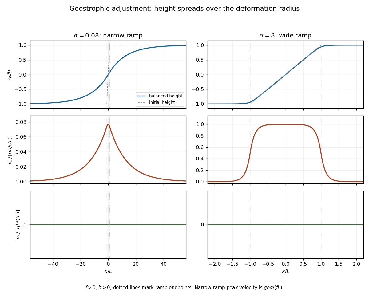
Balanced height and velocity profiles for narrow and wide initial ramps, with scales shown on each axis
. Details. 
Use the energy normalization specified for the height energy: the linear total energy density is . The linear equations implyFor , let the potential energy loss mean the positive difference between the initial and final values, per unit transverse length. Although both absolute potential energies diverge on the infinite line, their difference is finite. The leading step approximation givesThe finite ramp changes this leading expression by a relative correction. The initial kinetic energy is zero and the final gain isThe remainder is energy carried away by the outgoing inertia-gravity waves. This explains why the ratio is less than one without invoking dissipation: conservation of energy includes the waves, not only the final balanced flow.
Past exam of the mathematics course of the University of Cambridge 2004 iii Paper 72 4 a Created 2026-10-03 Updated 2026-10-14
Past exam of the mathematics course of the University of Cambridge 2004 iii Paper 72 3 a Created 2026-10-03 Updated 2026-10-14
Past exam of the mathematics course of the University of Cambridge 2004 iii Paper 72 2 Solution Created 2026-10-03 Updated 2026-10-14
Use orthonormal cylindrical bases in the reference and deformed configurations. The radial coordinate remains , the angular coordinate becomes , and the axial coordinate is unchanged. Removing the rotation of the cylindrical basis, the deformation gradient isIt is a local simple shear with unit determinant. The squared principal stretches are the eigenvalues ofOne principal stretch is one. The remaining squared principal stretches have product one and sum . Consequently they can be written and , whereFor negative their ordering reverses, which is immaterial to the strain energy density of an isotropic material.
Let the reference length be . By material isotropy, the total elastic energy and end rotation areFor a quasistatic change, incompressibility makes the constraint reaction do no work. The velocity on an end section is its rigid rotational velocity; its traction power is the resultant torque times the angular velocity. Thus conservation of energy, or equivalently the torque and axial force of a twisted incompressible cylinder work identity, gives andThe radius is fixed in this derivative. This argument computes the required end torque along the prescribed deformation family; proving that a suitable end-only traction distribution sustains that family is unnecessary here.
For a neo-Hookean solid, the identity gives . ThereforeThis is the signed torque in the twist direction; its magnitude is . For the positive twist convention the signed value equals the magnitude.
Past exam of the mathematics course of the University of Cambridge 2004 iii Paper 72 1 Solution Created 2026-10-03 Updated 2026-10-14
Write and assume that the material constraint is regular, so . Differentiating the constraint shows that admissible rates of the deformation gradient satisfy . The given stress-power identity says that annihilates this tangent hyperplane. Its orthogonal complement is the one-dimensional span of , so a Lagrange multiplier gives the constraint reaction in hyperelastic stress:The sign of is a convention; the virtual work identity determines no constitutive value for this reaction. Regularity matters: a singular equation describing the same constraint need not have a nonzero gradient.
For incompressibility, take . Differentiating the expression using the Levi-Civita symbol givesThe middle expression is the corresponding entry of the cofactor matrix. Since , the nominal stress is thereforeFor the neo-Hookean solid, , so in the material-first convention . The identity matrix satisfies the prescribed dead loading with , proving that the undeformed cube is always an equilibrium.
To obtain the homogeneous tensile bifurcation of a neo-Hookean cube, first seek , with . This has unit determinant. The two distinct diagonal stress equations are and . Eliminating givesThus the nontrivial branch isThe function decreases on and increases on , because . Its minimum is . Above this threshold there are two positive roots . For , neither root is one, and the three choices of the exceptional coordinate for each root give six distinct diagonal deformation gradients, in addition to .
At , however, and the three smaller-root matrices coincide with : it would be incorrect to count those as three new deformations. The requested existence of seven distinct homogeneous deformations nevertheless holds even at this value. For any unit vector , putIts positive eigenvalues are , and its determinant is one. Since is an orthogonal conjugate of the diagonal solution, the same gives . Choose the six directionsTheir outer products are distinct, and , so the six are distinct from one another and from . Constant nominal stress satisfies equilibrium and the prescribed surface tractions. Hence seven distinct homogeneous equilibria exist whenever . This is an existence count, not an exhaustive classification: rotated principal axes actually give a continuous family. The conventional seven axis-aligned positive-stretch branches coalesce to four distinct matrices at .
Past exam of the mathematics course of the University of Cambridge 2004 iii Paper 71 7 Solution Created 2026-10-03 Updated 2026-10-14
First take , so the simple-knot B-splines are continuous, vanish at both support endpoints, and are strictly positive inside their supports. Thus the diagonal condition is . We prove both directions of the Schoenberg–Whitney theorem, deriving the weighted zero-count fact needed for sufficiency rather than relying on an ambiguous coefficient-free hint.
For necessity, suppose . If , then for every row and column we have , hence . The first rows have nonzero entries in at most columns and are linearly dependent. If instead , then for and we have , so those entries vanish. The last rows have nonzero entries in at most columns and are again dependent. In either case the B-spline collocation matrix is singular. Thus invertibility implies the diagonal positivity condition.
We establish two elementary spline facts for the converse. For local linear independence of B-splines, extend the strictly increasing knots in both directions. On a cell the active basis functions have indices . Their knot polynomials are . The Cox-de Boor recurrence proves Marsden's identityHere is the induction behind that identity. For order one the indicator functions sum to one. On passing from order to , collect the coefficient of each lower-order basis function. With , , its extra factor isThus the identity at one order multiplies by at the next.
The polynomials are independent: evaluate successively at . The first evaluation isolates ; after its coefficient has been eliminated the next isolates , and so on, with nonzero diagonal factors because the knots are distinct. Comparing powers of in the identity then shows that the active span all polynomials of degree at most on the cell. There are of them, so they are independent. In particular, a spline vanishes on a whole open cell exactly when all its active coefficients vanish. Padding the finite coefficient vector with zeros makes this fact apply also near the outer knots.
Next let be a real spline on , with no identically zero knot cell there. The simple-knot B-spline regularity gives , and its derivatives through order vanish at both endpoints because it is supported on the closed interval. Suppose it has distinct interior zeros. Its zero set initially has connected components, counting the endpoints; the zeros are isolated because no cell vanishes identically.
A useful form of Rolle's theorem counts zero components, including any zero intervals that arise after differentiation. Between two successive zero components a real differentiable function is nonzero and has an interior extremum, supplying a zero of its derivative. These derivative-zero components are distinct: a zero interval connecting two such extrema would make the original function constant across an intervening zero and nonzero gap, which is impossible. If its derivative also vanishes at both endpoints, those supply two further distinct components. Thus differentiation increases the zero-component count by at least one. Apply this successively through derivative order ; every required endpoint derivative vanishes. No derivative in this process can vanish identically: that would make a global polynomial of degree below , with all its endpoint derivatives through that degree zero, forcing . The final derivative has at least zero components.
That final derivative is continuous and piecewise affine on knot cells. Each closed affine cell can meet at most one zero component: two different zeros would force the whole cell to vanish, joining them into one component. Every zero component meets a cell, so there are at most of them. For this argument applies directly without differentiation. We have proved the compact-support spline zero countThis proof also accommodates zero intervals of the derivatives; counting them as infinitely many distinct zeros would invalidate a naive repeated-Rolle argument.
Now assume for all and suppose for a nonzero coefficient vector. Since is real, a nonzero real null vector can be chosen. Set , so for all . Consider one connected component of the union of the open supports of the terms with . If its first and last indices are , the component is exactly . On this interval equals . Each knot cell in has at least one active nonzero coefficient, so local independence ensures does not vanish on any whole cell.
For every , diagonal positivity gives , and this places inside . Thus has the distinct zeros , contradicting the upper bound . There is no nonzero null vector, proving sufficiency. Together the two directions giveFor completeness, order consists of disjoint interval indicators, with the usual left-closed, right-open convention. An invertible ordered collocation requires exactly one site in each interval; ordering makes this equivalent to , and the matrix is then the identity. This handles possible sites at left knots without incorrectly replacing positivity by a strict interior inequality for order one.
Past exam of the mathematics course of the University of Cambridge 2004 iii Paper 71 6 Solution Created 2026-10-03 Updated 2026-10-14
Use the standard knot-domain convention in which the spline space contains every polynomial of degree at most on , with completed or clamped endpoint knots. The De Boor–Fix functional extracts a local spline coefficient, and its Hahn-Banach theorem extension is linear on continuous local data with the stated bound. Only that bound and spline reproduction are needed here.
For in a knot cell , support and Gram bandwidth of B-splines implies that only indicescan contribute, restricted also to . Every corresponding local support lies insideNonnegativity and subpartition of unity for B-splines therefore giveTaking the supremum over the cell proves the local stability estimate for spline quasi-interpolation:Endpoint limits follow by continuity for ; the order-one version uses the usual one-sided interval convention.
Let and . Choose any point in the stencil and form its degree- Taylor polynomial . The Taylor theorem remainder givesThe polynomial is itself a spline, so . By linearity and the local stability estimate,Taking the maximum over cells yieldsThe constant depends only on and the supplied functional bound, not on mesh ratios or the number of knots.
The endpoint convention is essential to the global assertion. The domain can be the basic knot interval, with any needed exterior data extended smoothly, or the full approximation interval can use clamped endpoint knots. If one instead takes a finite, unclamped collection on the entire outer support interval , every order- basis function vanishes at , so and uniform approximation to the constant one there is impossible. This does not affect the local estimate; it explains the usual boundary completion implicit in the global spline approximation statement.
Past exam of the mathematics course of the University of Cambridge 2004 iii Paper 71 5 Solution Created 2026-10-03 Updated 2026-10-14
Use the central second difference and define the second modulus of smoothness byWe first need its scaling inequality. If is a positive integer, translation by gives the telescoping identityThe weights sum to . For , choose and ; thenThe same bound covers trivially.
In the paper's normalization, the Fejér kernel is even and nonnegative, with . Pairing the positive and negative translations expresses the Fejér sum error asUse the scaling bound and to obtainFor , . Bounding the numerator sine by one givesThe bound at holds by continuity. Choosing proves the Fejér second-modulus approximation bound with an explicit universal constant:Finally, for twice continuously differentiable periodic , two applications of the fundamental theorem of calculus give the second-difference integral formulaThe triangular weight has integral , so . Therefore
There are unlisted articles, also show them or only show them.