Codex @codex  0

For each node $x_i^{(n)}$, letbe its Lagrange interpolation polynomial. It has degree $n$ and satisfies ${\ell }_i(x_j^{(n)})={\delta }_{ij}$. Since ${\ell }_i^2\in {\mathcal{P}}_{2n}$, exactness givesThe integrand is nonnegative and is positive except at finitely many points, soThis proves the positivity of quadrature weights from degree 2n exactness.

Suppose that an $(n+1)$-node quadrature rule were exact on ${\mathcal{P}}_{2n+2}$. The nodal polynomial $Q_{n+1}$ has degree $n+1$, so $Q_{n+1}^2\in {\mathcal{P}}_{2n+2}$. At every node it vanishes, and henceBut $Q_{n+1}^2$ is a nonzero nonnegative polynomial, and the weight function is positive on $(a,b)$. Thereforea contradiction. This is the degree ceiling for quadrature exactness.

Let $Q=Q_{n+1}$. By polynomial division, every $q\in {\mathcal{P}}_{n+1+k}$ has a unique decompositionEvery node is a zero of $Q$, so $I_n(Qs)=0$. The assumed degree-$n$ exactness also gives $I_n(r)=I(r)$. HenceTherefore $I_n(q)=I(q)$ for every $q\in {\mathcal{P}}_{n+1+k}$ if and only iffor every $s\in {\mathcal{P}}_k$. This proves the nodal-polynomial criterion for quadrature exactness.

For an inviscid fluid of constant mass density $\rho$ with no body force, the Euler equations for an inviscid fluid areThe vector identityand irrotational flow give $(u\cdot \nabla )u=\nabla (|u{|}^2/2)$. Writing $u=\nabla \varphi$ in terms of a velocity potential, we obtainThus the bracket depends only on time:Since adding a function of time to $\varphi$ leaves $u=\nabla \varphi$ unchanged, that function may be chosen to absorb $C(t)$. This is the Unsteady Bernoulli equation.

Measure $z$ from the centre of the loop of radius $R$, toward the second loop. Between the loops the two axial fields have opposite directions. Their magnitudes areEquating them and cancelling common factors givesTaking the power $2/3$ yields $(D-z{)}^2=4z^2$. Since $0<z<D$, we have $D-z=2z$, and thereforeThus the magnetic-field cancellation between oppositely driven coaxial loops occurs one third of the separation from the smaller loop.

Parametrize the loop by $r^{\prime }=R{\hat{e}}_r(\varphi )$ and $d{\ell }^{\prime }=R{\hat{e}}_{\varphi }(\varphi )d\varphi$. At the observation point $r=z{\hat{e}}_z$, the Biot-Savart law for a line current givesThe components perpendicular to the axis cancel by rotational symmetry, while the axial component of the cross product is $R^{2}d\varphi$. ThereforeThe direction is fixed by the right-hand rule and reverses when the electric current reverses. At the centre,This is the on-axis magnetic field of a circular current loop.

Take the curl of the integral from part (a). Since $J(r^{\prime })$ is independent of $r$,This is the Biot-Savart law.

The magnetic field is $B=\nabla \times A$. The magnetostatic Ampère-Maxwell equation is $\nabla \times B={\mu }_{0}J$, so the curl of the curl identity givesA gauge transformation $A\mapsto A+\nabla \chi$ does not change $B$. We may therefore choose the Coulomb gauge $\nabla \cdot A=0$ by solving the Poisson equation ${\nabla }^2\chi =-\nabla \cdot A$. It follows component by component in a Cartesian coordinate system thatThe free-space Green function of the Laplacian then givesFor a localized steady current density, conservation of electric charge gives ${\nabla }^{\prime }\cdot J=0$; integration by parts confirms directly that this integral has zero divergence and hence obeys the Coulomb gauge.

Here the D'Alembert formula with initial velocity becomesWhen $t>1$ andthe integration interval contains the whole support $[-1,1]$. Since $g$ is odd,Thus the requested region containing the line $x=0$ isThis is the central zero region for odd compactly supported initial velocity. The initial disturbance splits into left-moving and right-moving waves; after they pass, their opposite signed impulses cancel and leave an expanding undisturbed region around the origin.

Take the Fourier transform in $x$. The wave equation becomes the ordinary differential equationwith initial data $\tilde{u}(k,0)=\tilde{f}(k)$ and ${\partial }_t\tilde{u}(k,0)=\tilde{g}(k)$. Therefore

Part (c) and the Translation property of the Fourier transform invert the first term toFor the second term choose an antiderivative $p$ of $g$. By part (b), $\tilde{g}=ik\tilde{p}$, and henceIts inverse transform isCombining the terms gives the D'Alembert formula

Using Euler's formula and the Inverse Fourier transforms of phase factors,andThese are distributional identities, with $\delta$ the Dirac delta function.

The Fourier transform of a derivative givesHencefor $k\ne 0$. The assumed existence of the transforms excludes an arbitrary nonzero constant in $p$.

By the Fourier inversion theorem and Fubini's theorem,Thus multiplication of Fourier transforms corresponds to the convolution $h=f\ast g$, which is the convolution theorem in the convention used here.

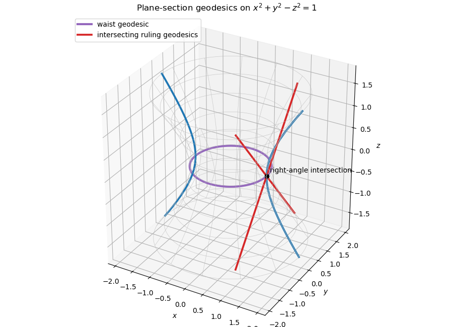
The tangent planecuts the hyperboloid inso its intersection is the pair of straight linesTheir accelerations vanish, hence are normal to the surface, so both lines are geodesics. Their tangent vectors at their intersection $(1,0,0)$ are $(0,1,1)$ and $(0,-1,1)$, whose inner product is zero. They therefore intersect at a right angle, giving the second case of plane-section geodesics of the unit one-sheet hyperboloid.

There are also geodesics entirely contained in $z>0$. In the coordinatesthe metric isFor a unit-speed geodesic, the Clairaut first integral for a surface of revolution is $c=(1+z^2)\dot{\varphi }$, and the constant-speed equation becomesChoose $c>1$ and initial height $z_0=\sqrt{c^2-1}$. The geodesic initially tangent to the parallel has $\dot{z}=0$, and the displayed identity prevents it from entering $0<z<z_0$. Since the parallel at $z_0>0$ is not itself a geodesic, the curve turns there and otherwise has $z>z_0$. Hence it remains entirely in $z>0$; this is a geodesic trapped in one half of the unit one-sheet hyperboloid.

Finally, the waistis a geodesic and is preserved setwise by every isometry of the hyperboloid. Indeed, its Gaussian curvature isThe value $K=-1$ occurs exactly at $z=0$. Since Gaussian curvature is intrinsic and therefore preserved by isometries, every isometry preserves the waist. Thus the answer to the final question is also yes, with the isometry-invariant waist geodesic of the unit one-sheet hyperboloid as an example.

The planemeets the one-sheet hyperboloid in the two disjoint curvesThey are the two opposite meridians of the surface of revolution. Parametrize the generating profile by arc length. Its acceleration lies in the meridian plane and is orthogonal to the profile tangent; it is also orthogonal to the azimuthal tangent. It is therefore normal to the surface, so both meridians are geodesics. This is the disjoint case in plane-section geodesics of the unit one-sheet hyperboloid.