
Power law Created 2026-09-24 Updated 2026-10-13
A power law is a relation , with fixed constants and . For positive , any real number is allowed. Its useful feature is a simple scaling rule:The same proportional change of input produces the same proportional change of output, independently of the starting value. The exponent controls that response; the coefficient fixes the magnitude.
For example, the area of a circle is . Doubling the radius multiplies its area by four, and tripling it multiplies the area by nine. The volume of a sphere is : the same changes multiply its volume by eight and twenty-seven. The distinction explains why similarly shaped objects do not preserve their ratio of surface area to volume when their size changes.
When the output is positive, a logarithm turns the power law into a straight-line relation. Using positive reference values and ,These ratios are dimensionless quantities, so the formula also applies to physical measurements with units. Plotting both ratios on a logarithmic scale gives a line of slope . Changing a unit changes the numerical coefficient, while the exponent stays the same. Positive describes increasing values; negative describes decreasing values; gives a constant. The zero coefficient is a degenerate case with no useful logarithmic slope.
Exact scaling is stronger than regular variation. The function has a doubling ratio tending to four, but its logarithmic correction keeps growing. The diagram contrasts it with the exact power law .
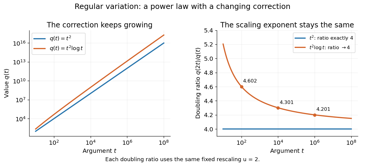
Exact quadratic scaling and a logarithmic correction have different finite doubling ratios, even though the correction leaves the limiting exponent unchanged
. Details. 
A power law for a probability density and a power law for a tail probability have different exponents. For a Pareto distribution with and lower endpoint one,The tail probability has exponent ; differentiating it and changing sign gives the probability density exponent . Confusing them changes the interpretation of a fitted exponent. The normalizing coefficient and lower endpoint also matter: a decreasing power law is not automatically a valid probability density over the entire positive real line.
The appearance of a line over a finite logarithmic range is evidence to investigate, rather than a proof of an exact power law or its mechanism. In their study of power-law distributions, Clauset, Shalizi and Newman combine maximum likelihood estimation, goodness-of-fit tests and comparisons with alternative models; their abstract explains why ordinary least-squares fitting can give misleading results for tail data. See Aaron Clauset, Cosma Rohilla Shalizi and M. E. J. Newman, Power-law distributions in empirical data, SIAM Review 51 (2009), 661–703. The scaling rule is mathematically exact when it defines a model; whether a dataset supports that model is a question of statistical inference.
Noncommutative algebra Created 2026-09-24 Updated 2026-10-18
Noncommutative algebra studies rings whose multiplication need not commute and their one-sided ideals and modules.
Commutative algebra Created 2026-09-24 Updated 2026-10-18
Commutative algebra studies commutative rings, ideals, modules, and the spectrum of a ring. Its basic question is which familiar rules of integer and polynomial arithmetic survive in a new setting. The distinction between units, zero divisors, and integral domains makes that question concrete.
Homogeneous polynomial Created 2026-09-24 Updated 2026-09-24
Group theory Created 2026-09-24 Updated 2026-10-14
A group records reversible operations that can be combined consistently. Group theory studies their subgroups, group homomorphisms, group actions, and quotient groups. A symmetry group makes the abstraction visible: transformations may change individual points while preserving a specified object or its structure. An orbit of a group action records which positions can be exchanged, while a stabilizer subgroup records which operations leave a selected feature fixed.
Fundamental theorem of algebra Created 2026-09-24 Updated 2026-10-13
Every nonconstant complex polynomial has a complex root and therefore factors completely into linear factors over .
Unit in a ring Created 2026-09-24 Updated 2026-10-03
Unique factorization domain Created 2026-09-24 Updated 2026-09-24
Transcendental number Created 2026-09-24 Updated 2026-09-24
Surjective function Created 2026-09-24 Updated 2026-10-13
Star-shaped set Created 2026-09-24 Updated 2026-09-24
Smith normal form Created 2026-09-24 Updated 2026-09-29
For every matrix over a principal ideal domain, there are invertible matrices such thatThe nonzero diagonal entries are unique up to multiplication by units. Over the integers, and are unimodular and the may be chosen positive; their products are the greatest common divisors of the -rowed minors.
Root of unity Created 2026-09-24 Updated 2026-10-03
RSA cryptosystem Created 2026-09-24 Updated 2026-10-06
Polynomial interpolation error Created 2026-09-24 Updated 2026-10-13
Pigeonhole principle Created 2026-09-24 Updated 2026-10-18
Place objects into boxes, assigning each object to exactly one box. Here is a nonnegative integer and is a positive integer. The pigeonhole principle says that if , some box contains at least two objects. Equivalently, a function from an -element finite set to an -element finite set cannot be an injective function when . The boxes may stand for categories rather than physical containers. [ref]
https://ocw.mit.edu/courses/6-042j-mathematics-for-computer-science-spring-2015/mit6_042js15_textbook.pdf#page=581. Lehman, Leighton and Meyer, Mathematics for Computer Science, section 14.8, rule 14.8.1
For thirteen objects and twelve boxes, a box containing at least two is unavoidable. Thinking of thirteen people and their birth months gives the same conclusion: at least two share a birth month. Twelve people could occupy the twelve months one apiece, so thirteen is the smallest number that forces a shared month. The generalized pigeonhole principle quantifies how many objects must share a box when there are still more objects.
The useful surprise is that the pigeonhole principle proves existence without needing to locate the objects involved. Choosing a good assignment rule is often the creative step: equal labels can mean equal remainders, nearby points, or repeated states of an algorithm. Once the rule is chosen, a short count can force a relationship among a much larger collection of objects. The pigeonhole principle itself does not name the crowded box. When the objects and their assignments are explicitly available, a simple algorithm finds one: scan the objects, keep the first object seen in each box, and stop when a later object enters an occupied box. At most scanned objects are needed when .
A geometric example. Any five points in a square of side one contain two whose Euclidean distance is at most . Give each point Cartesian coordinates . Divide both ranges into the intervals and , making four cells. Thus belongs to the left half and to the right half; belongs to the lower half and to the upper half. This convention assigns every boundary point to exactly one cell.
The pigeonhole principle puts two of the five points in the same cell. Their differences in Cartesian coordinates have magnitude at most , so the Pythagorean theorem gives their Euclidean distance the boundFor the plotted points , , , and , the first two occupy the lower-left cell and have Euclidean distance . These Cartesian coordinates exhibit the forced pair; the argument applies to every placement of five points.
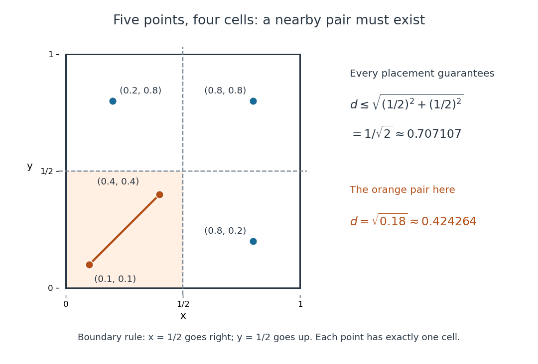
The pigeonhole principle places two of five points in one of four cells of a square, bounding their Euclidean distance by
. Details. 
An arithmetic example. Assign eight integers to their seven residue classes modulo the integer modulus . The pigeonhole principle gives two with the same residue class, so is an integer divisor of their difference. In , for example, and satisfy the integer congruence , and . Likewise, assigning fractional parts to short intervals gives the Dirichlet approximation theorem; its existing article explains the approximation bound.
Noetherian ring Created 2026-09-24 Updated 2026-10-06
Nilpotent polynomial Created 2026-09-24 Updated 2026-09-24
Minimal number of generators Created 2026-09-24 Updated 2026-10-13
Mathematical induction Created 2026-09-24 Updated 2026-10-14
A mathematical induction proof establishes a property for every integer by proving its induction base case and its inductive step. If a counterexample existed, the well-ordering principle would give a least one; its predecessor and the inductive implication exclude it. The starting case excludes a counterexample at .
The useful idea is to cover infinitely many cases with two finite pieces of reasoning. The induction base case starts the chain, and the inductive step shows that success at an arbitrary stage propagates to the next. It is especially natural when a construction adds one item at a time: another row of a diagram, another input processed by an algorithm, or another term of a sequence. The loop invariant method is the same propagation idea applied to successive stages of a computation.
For the triangular number , the proposed formula is . At , both sides are one. Assuming the formula for a fixed positive integer , add the next row:This is the desired formula at , proving the inductive step. For example, and ; these numerical cases illustrate the general step rather than replace it.
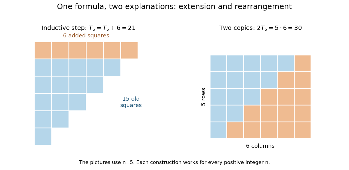
Adding the next row gives the induction step; rearranging two triangular arrays gives the same formula geometrically
. Details. 
The second picture explains where the formula comes from: two copies of the triangular arrangement tile an by rectangle. Thus . The mathematical induction argument certifies how the formula continues, while the rearrangement makes its factors visible. Neither picture is restricted to the five rows drawn: both constructions are specified for every positive integer .
There are unlisted articles, also show them or only show them.