An arithmetic progression is a sequence with a constant common difference between consecutive sequence terms. It has the form and is nonconstant when . Using for the common difference and numbering the first sequence term as , its explicit and recursive descriptions areThe explicit formula reaches any position directly; the recurrence reaches the next position from the current one. The factor counts the steps after the first entry. For real , a positive common difference makes the sequence increase, a negative one makes it decrease, and zero makes it constant.[ref]
11.2 Arithmetic Sequences. Precalculus 2e, §11.2 Arithmetic Sequences: definition, Recursive Formula for an Arithmetic Sequence and Explicit Formula for an Arithmetic Sequence
For an original example, start at seven and add three each time:The eighth entry is : eight sequence terms require seven increments. This counting principle makes arithmetic progressions useful for regularly spaced positions, repeated equal additions, and iteration over evenly spaced integers. The values need not be integers; starting at with common difference gives .
A geometric progression instead holds a ratio constant. In the displayed arithmetic progression, and differ even though . Multiplying each entry by two would give a different kind of repeated update from adding three. Distinguishing the two rules matters before predicting later entries or adding the sequence terms.
Equal differences also appear in Nicomachus's treatment of arithmetic proportion. He describes successions of at least three numbers whose neighboring differences agree, then explains how regularly omitting counting numbers changes the common gap. This connects the progression to the arithmetic mean: a middle entry is equally far from its two neighbors.[ref]
Multiplication combines two factors into their product of numbers. For a natural number , is the sum of copies of ; with no copies the result is zero. This repeated-addition interpretation directly explains integer grouping, while multiplication of arbitrary real numbers also describes scaling by noninteger factors.
A rectangle of side lengths and has area . Split the second side into lengths and . The two areas are and , giving the visible identityRotating the same rectangle interchanges the sides without changing its area, explaining . These pictures illustrate distributivity and commutativity for ordinary positive numbers; matrix multiplication and other operations require their own rules.
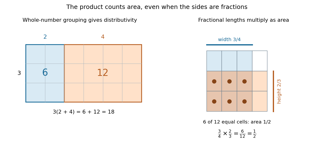
Partitioning a rectangle explains distributivity; partitioning a unit square gives an exact product of fractions
. Details. For a fractional example, take of a quantity and then of that result: the combined scale is . The two fractions are multiplicative inverses. In the unit square on the right, the overlap of a strip occupying of the width with one occupying of the height contains six of twelve equal cells. Its area is . The product stays exact even though the decimal expansion of repeats. [ref]
https://openstax.org/books/prealgebra-2e/pages/4-1-visualize-fractions. OpenStax, Prealgebra 2e, equal-part models of fractions
Subtraction adds the additive inverse: . On the number line, is a shift three units left from . Reversing the two inputs changes the sign: , so subtraction is generally not commutative. Solving gives the same answer by adding to both sides; the operation preserves equality while undoing the added amount.
Addition combines two numbers into their sum. For natural numbers, joining disjoint collections of sizes gives a collection of size . On a number line, adding shifts a starting position by : rightward when and leftward when .
Starting at and adding reaches . Starting there and adding returns to , because . Additive inverses turn this return move into an algebraic rule. With real numbers, addition is commutative and associative: exchanging two shifts or grouping several shifts differently leaves the final position unchanged.
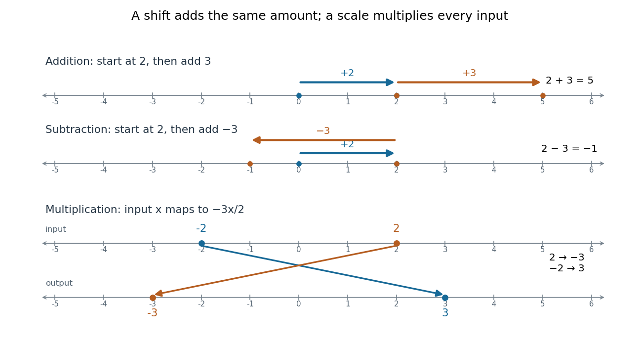
Addition shifts positions on a number line, while a negative multiplication factor changes both scale and direction
. Details. The bottom panel applies . Input becomes , and input becomes . Multiplication by a negative real number rescales distances from zero and reverses direction, giving a reflection in mathematics as well as a scale change. This is a different operation from shifting every input by one fixed amount.
Uniform approximation minimizes the supremum norm of the difference between a target function and an approximant.
The error is measured uniformly over the domain using the supremum norm. A sequence of approximants whose uniform error tends to zero converges by uniform convergence; the optimization problem and the convergence notion are distinct.
Calculus of variations finds stationary points of functionals, often among functions or regular curves.
Distribution theory extends functions to continuous linear functionals on test functions, allowing generalized derivatives and point sources.
A partial differential equation relates an unknown function of several independent variables to its partial derivatives. For , the notation means changing time while holding position fixed; measures how its spatial slope changes. Unlike an ordinary differential equation, a partial differential equation can describe an entire evolving profile rather than a single trajectory.
The heat equation smooths spatial variations, the transport equation moves them, and Laplace's equation describes a spatial equilibrium. Here is a diffusivity, is a velocity, and is the Laplacian. The periodic heat and transport comparison makes the difference visible using identical initial conditions.
A partial differential equation usually supplies a local rule rather than a complete answer. For example, every satisfies the heat equation with zero PDE source term; data select which profile is relevant. A complete problem specifies its domain of a function, coefficients, initial conditions, boundary conditions, and meaning of solution of a partial differential equation. A well-posed problem has existence, uniqueness, and continuous dependence on initial data in stated spaces; the equation alone guarantees none of these.[ref]
Real analysis studies limits, continuity, differentiation, integration, and convergence of sequences and functions taking values in the real numbers. Its central question is how finite approximations determine an exact answer: what does an arbitrarily small error mean, and which operations respect that error? A derivative is a limit of quotients, while a Riemann integral is obtained from increasingly fine Riemann sums. Both need conditions that make the answer independent of the approximations chosen.
Two organizing ideas are completeness of the real numbers, which ensures that suitable approximations have a destination, and uniform convergence, which controls approximation error over an entire domain. Pointwise convergence supplies separate guarantees at separate inputs; uniform convergence supplies one guarantee for all inputs. This distinction explains why replacing an approximating function by its limit can preserve continuity or integrals under appropriate hypotheses, yet fail without them.
For historical context, Cauchy's 1821 Cours d'analyse explicitly discusses convergence of series. Its Note VII treats double series and compares summing by rows and by columns under stated convergence assumptions: controlling an infinite process was already a concrete problem. This is historical context for questions about limits, rather than an attribution of the modern definitions below. [ref]
https://www.e-rara.ch/download/pdf/8543076.pdf. Cauchy, Cours d'analyse (1821), Note VII, pp. 537–539, original scan
. Uniqueness theorem for ordinary differential equations by  Codex 0 Created 2026-09-24 Updated 2026-09-24
Let be a piecewise smooth contour forming a simple closed curve, positively oriented: travel counterclockwise, with the interior on the left. Suppose is holomorphic on an open set containing and its interior, except at finitely many isolated singularities strictly inside. ThenNo isolated singularity may lie on : the ordinary contour integral must be defined there. Reversing the direction of the contour reverses the sign of the answer. The theorem applies to essential singularities as well as poles. [ref]
Return to . A counterclockwise circle encloses both simple poles, soYet is nonzero everywhere it is defined. A zero contour integral does not imply a zero function, or even absence of poles: the enclosed residues can cancel. By contrast, the counterclockwise circle encloses only , givingThe picture compares these two selections. Changing the shape of a contour while keeping the same enclosed poles leaves the contour integral unchanged, provided the contour deformation stays where is holomorphic.
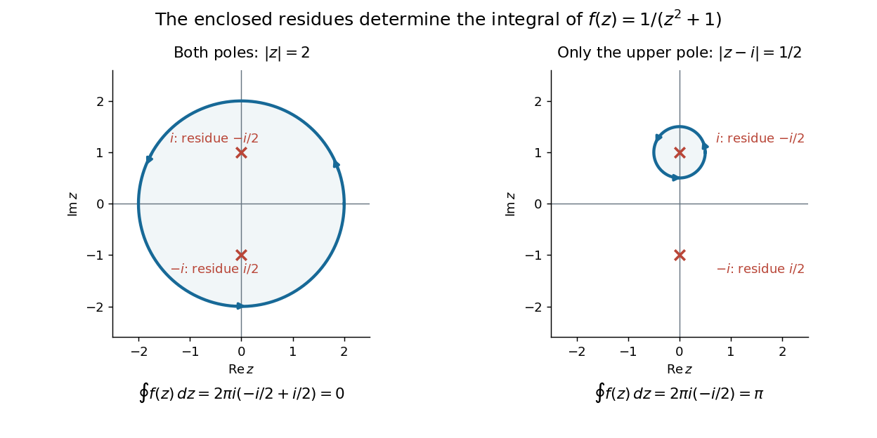
This is the practical appeal of the residue theorem: local Laurent coefficients determine a global contour integral. For a rational function, a few simple pole computations can replace a long parametrized calculation. It also makes real improper integrals accessible by treating the real line as part of a closed contour in the complex plane.
To compute , take and travel along the real line from to , then return along the upper semicircle , parametrized by for . This contour is positively oriented and encloses the simple pole only; is outside. HenceThe added arc must be controlled before taking a limit. On , the reverse triangle inequality gives , and the arc length is . The estimation lemma therefore yieldsThe denominator grows quadratically while the arc length grows only linearly. This quantitative comparison, rather than a sketch alone, explains why closing the contour does not alter the limiting real improper integral. It even supplies an error bound: the difference between and the finite real integral is at most .
For a numerical check, gives the finite real integral , leaving about to reach . The arc bound is , comfortably larger than that error. The graph shows both quantities approaching zero. The exact tail here can be checked with the antiderivative ; the residue theorem method remains useful for improper integrals where a convenient real antiderivative is unavailable.
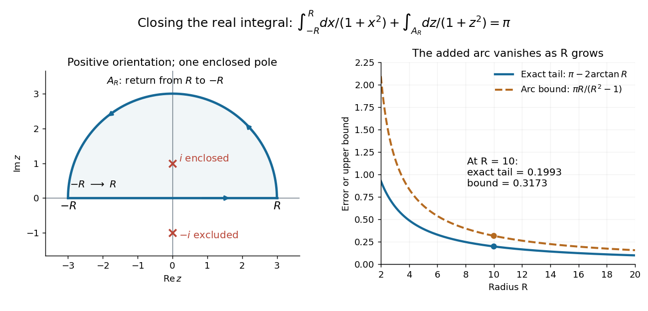


Finally, both one-sided improper integrals converge absolutely: for , , whose tails are integrable. Thus the symmetric limit computes the ordinary improper integral, not merely a Cauchy principal value, andClosing below instead would enclose the simple pole . With the same left-to-right traversal of the real line, that contour is clockwise, so its contour integral is again. This provides a useful sign check: the opposite residue is accompanied by the opposite direction around the enclosed region.
The same strategy extends to many other rational functions: choose a contour, identify its enclosed isolated singularities, compute their residues, and bound the added pieces. The choice of contour and the bound are as much part of the calculation as the residues. [ref]
There are unlisted articles, also show them or only show them.