
The instantaneous acoustic energy flux is for linear acoustics. Its time average is the sound intensity.
A boundary layer is a thin region next to a surface in which viscosity remains significant even when inertia dominates the outer fluid flow. Its simplest example is laminar flow along a stationary flat plate: the no-slip boundary condition imposes zero velocity at the plate, while the outer velocity is . The resulting thin velocity profile contains a large normal velocity gradient, so small dynamic viscosity can still produce appreciable wall shear stress. The Blasius boundary layer makes this competition quantitative and explains how a plate aligned with the incoming fluid flow acquires drag.
The same balance appears in a singular perturbation of a differential equation: large derivatives in a thin region can keep a term with a small coefficient significant. For on with and , the inner variable resolves a left boundary layer of width .
The Rayleigh-Taylor instability occurs when a denser fluid lies above a lighter fluid in a gravitational field, causing interface perturbations to grow.
Mass conservation states that matter is neither created nor destroyed. For mass density and velocity , its local form is .
The continuity equation expresses local conservation as time change plus flux divergence equal to zero.
Energy flux is the energy crossing a unit area per unit time. For a one-dimensional inviscid gas with internal-energy density , it is
Compton scattering redistributes photon energy and momentum in a collision with a charged subatomic particle, here an electron. For a free electron initially at rest in the chosen inertial frame, an incident photon of energy leaves with energy after deflection through . The angle is between the incident and outgoing photon directions; it is not the electron recoil angle. Four-momentum conservation giveswhere is the electron rest mass and its final kinetic energy. The photon energy loss pays for the electron recoil: neither energy nor momentum disappears.
For an original worked example, stipulate , the rounded electron rest energy , and the rounded Compton wavelength ; means electronvolts. Treat these rounded inputs as the example's constants. They give the following calculated values, with energies rounded to three decimal places:
| Photon deflection | Outgoing photon energy in | Electron kinetic energy in | Wavelength increase in |
|---|
Since , every outgoing photon has and . At zero deflection there is no recoil; backscattering transfers the most energy. At fixed , the absolute wavelength increase is independent of incident energy, while the fractional energy loss grows with . This makes Compton scattering useful for inferring energy transfers from directions in photon detectors.
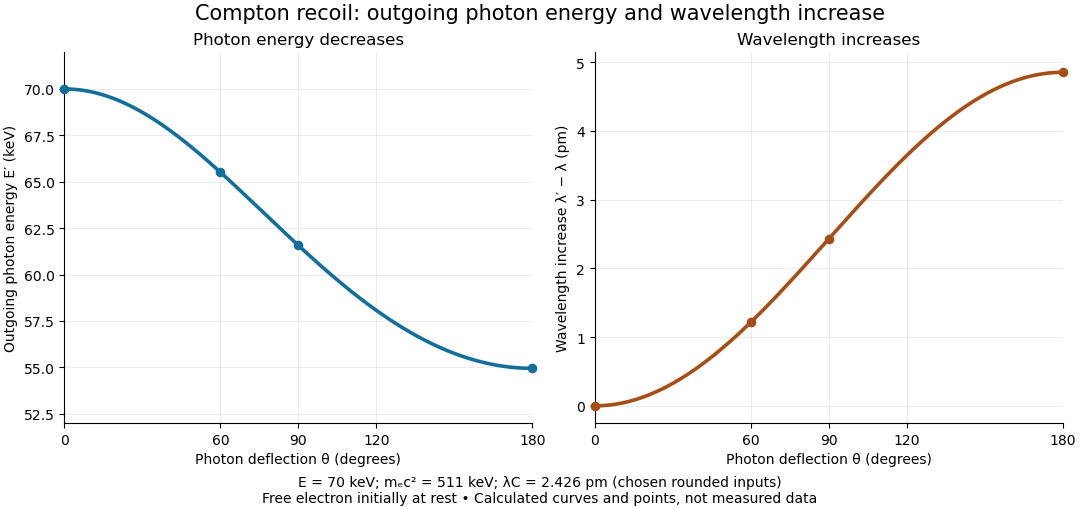
The free-electron-at-rest assumption matters. An electron in a bound state has binding energy and an initial momentum distribution. Neglecting these is useful when the transferred energy is large compared with the relevant binding energy and the initial momentum is small compared with the resolved momentum transfer. Otherwise the outgoing photon energies can broaden or depart from the stationary-target formula; an initially moving electron can even give energy to the photon.
A material may also scatter X-rays through a coherent elastic scattering channel with an effectively unshifted component. When an intact chemical atom of mass takes the recoil, the corresponding Compton wavelength is much smaller than the electron value. The single free-electron curve does not predict that component's weight. More generally, energy versus angle is a kinematic constraint; angular wave intensity requires a differential scattering cross-section, together with target and detector information.
Ramsey theory studies configurations that every finite coloring of a sufficiently large structure must contain. Its striking message is that some order is unavoidable even when no organized construction was used. A basic example is the Ramsey number for triangles: color every edge of a complete graph on six vertices red or blue, in any way, and some triangle in a graph has all three edges the same color. Five vertices do not suffice.
The objects receiving colors matter. In the Ramsey number for triangles, colors belong to edges, which represent all unordered pairs of distinct vertices; the vertices themselves have no colors. In the finite Ramsey theorem, colors can instead belong to all -element subsets of a finite set. A monochromatic set or homogeneous set for a colouring expresses agreement among the appropriate colored objects.
Why is this useful? Ramsey theory provides existence guarantees in combinatorics that survive every possible assignment of a fixed finite number of colors. The Ramsey theorem turns this into a structural dichotomy: every sufficiently large graph contains a large clique or a large independent set. In arithmetic, the Van der Waerden theorem guarantees monochromatic arithmetic progressions. The beauty is the universal quantifier: an adversary can choose every color and still cannot prevent the promised configuration.
These guarantees concern precisely specified configurations under stated hypotheses. They do not justify selecting arbitrary patterns in empirical data after seeing the data, or attributing statistical significance to a selected pattern. A mathematical guarantee of some monochromatic configuration alone says nothing about the empirical meaning of that configuration.
The subject's name comes from F. P. Ramsey's [ref]. The [ref]
https://www.cs.umd.edu/~gasarch/BLOGPAPERS/ramseyorig.pdf. original paper, pp. 264-268, Theorems A and B
records receipt on 28 November 1928 and presentation on 13 December 1928. Ramsey introduced the Ramsey theorem for r-sets and finite Ramsey theorem as tools for a problem in mathematical logic, while recognizing their independent interest in combinatorics. He also distinguished proving that a finite threshold exists from finding its smallest value, the quantitative question captured by a Ramsey number.Analysis of Boolean functions studies real-valued functions on a Boolean hypercube using Fourier analysis, probability theory, and combinatorics.
A permutation of a set is a bijection : every element has exactly one image and every element appears exactly once as an image. For a finite set, a permutation can also be recorded as an ordering of all its elements, once a reference order has been chosen. For three distinct letters , the six orderings areThere are three choices for the first letter, two unused letters for the second, and one for the third. Every path in the tree gives one complete ordering, and every ordering has one such path, so the rule of product gives , a factorial.
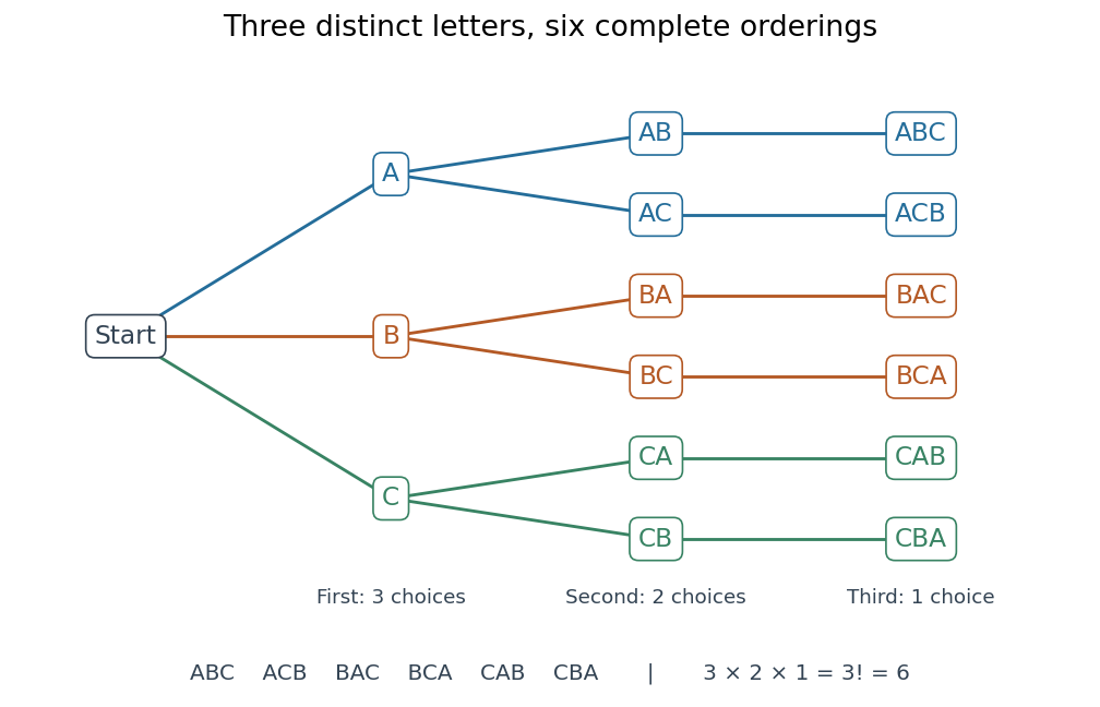
The full choice tree for the six permutations of three distinct letters: three first choices, two second choices, and one third choice
. Details. Ordering versus mapping. Label the reference positions . An ordering tuple of these labels describes the function ; conversely, reading the images recovers the ordering. For example,means , , , . Its ordered image list is , whereas its cycle decomposition of a permutation is : starting at , follow its successive images back to . Parentheses in the latter expression encode arrows around a permutation cycle, rather than an image list in reference order. [ref]
https://math.mit.edu/~fgotti/docs/Courses/C.%20Combinatorial%20Analysis/11.%20Permutations%20I/Permutations%20I.pdf. Felix Gotti, MIT 18.211, lecture 11, pages 1–2: arrangements, bijections and cycles
The two viewpoints answer different useful questions about the same object. An ordering tells us which object occupies each position; a bijection tells us where each label is sent and allows successive rearrangements through function composition. All permutations of labels form the symmetric group, whose subgroups are permutation groups. The counting viewpoint supplies possibilities, a factorial; the mapping viewpoint reveals how rearrangements combine.
Composition convention. Apply the rightmost permutation first:For the displayed and the transposition , direct evaluation givesFor instance, , but . Thus function composition of permutations need not be commutative; the omitted labels in these permutation cycles are fixed points.
The grid graph has vertices in the Cartesian power and joins two vertices when they differ by one in exactly one coordinate.
For finite sets , the cardinality of their union isAdd the individual cardinalities, subtract pairwise intersection counts, add triple intersection counts, and continue alternating. This is useful whenever one object can satisfy several conditions: a search result can match several filters, or a permutation can have several forbidden fixed points.
Among the integers from 1 to 30, let contain the multiples of 2 and the multiples of 3. Then , , and , because their common multiples are the multiples of 6. The naive sum counts those five twice; the correct union size is . The regions contain ten in alone, five in both, five in alone, and ten in neither.
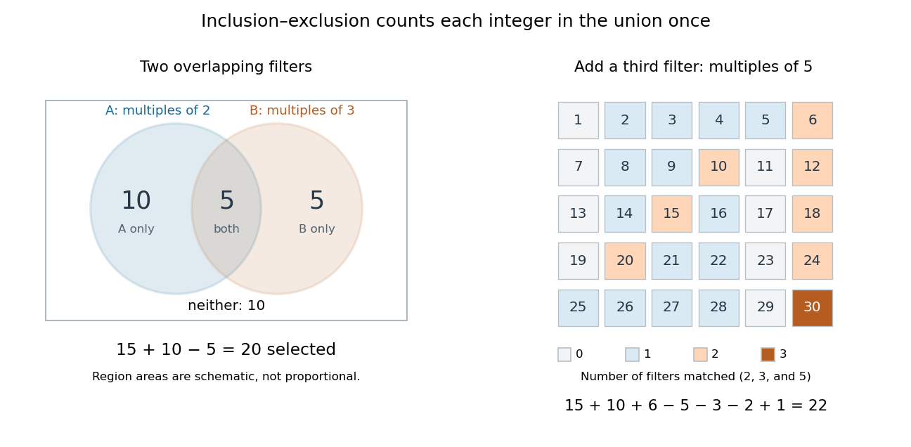
Subtracting overlap counts each selected integer once; a third divisibility condition requires adding the triple overlap back
. Details. Add a third set containing the multiples of 5. Its size is 6; the three pairwise intersections have sizes ; and the triple intersection contains only 30. The inclusion-exclusion principle gives integers divisible by at least one of 2, 3, and 5.
The alternating corrections have a local explanation. An object belonging to exactly of the sets is counted times, by the binomial theorem applied to . An object in none contributes zero. Thus overlapping descriptions are repaired without requiring the sets themselves to be disjoint. For probability, the same calculation applies to event probabilities in place of cardinalities, giving the inclusion-exclusion principle for probabilities.
Splitting an alternating permutation at its maximum giveswhere counts up-down permutations and complementation identifies up-down with down-up permutations.
For nonnegative integers and , the binomial coefficientcounts the -element subsets of an -element set. To obtain the formula, first choose an ordered list of different members in ways. Each subset appears in exactly orders, so divide by that factorial. The cases and each have one selection, the empty set and the whole set. For integer outside , the combinatorial convention is .
For , , the calculation is . The left-hand panel lists all ten subsets of . Marking an included member with one and an excluded member with zero gives a bijection with length-five binary strings containing exactly two ones. More generally, this makes selection, binary encoding, and coefficients in a binomial theorem three descriptions of the same count.
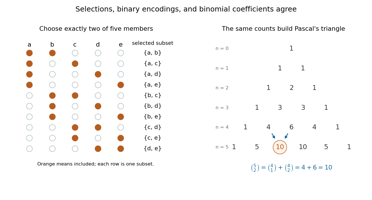


For a uniformly chosen two-person team, a specified person belongs to four of the ten teams, so the probability of their inclusion is . Uniform selection of a -element subset similarly gives inclusion probability for each member when , as the double counting identity shows.
For a nonnegative integer , the factorial is the product of the positive integers from to , with the empty product equal to :Thus , , , and . The factorial counts the permutations of distinct objects: arranging gives exactly . The choice tree in permutation shows the three choices for the first position, two for the second, and one for the last.
The value has a counting explanation: the empty set has exactly one ordering, the empty list. Equivalently, it has exactly one bijection to itself, the empty function. There are no choices to make, and one completed outcome. The factorial therefore obeys the recurrence relationThe useful distinction is how many positions are filled. For integers , choosing and ordering distinct objects by sampling without replacement gives the falling factorial, while choosing an unordered -element subset gives the binomial coefficient:For five people, assigning captain and deputy gives outcomes; choosing a two-person team gives . Every team has exactly assignments of the two roles, explaining the division. When , both counts are one. The factorial is useful here because one count of full orderings yields both formulas by cancellation and by forgetting order. [ref]
https://openstax.org/books/college-algebra-2e/pages/9-5-counting-principles. OpenStax, College Algebra 2e, section 9.5: counting ordered selections and combinations
Distinctness matters. If the two copies of in are indistinguishable, the visible arrangements are just , numbering . Temporarily labelling them gives six permutations, but exchanging the two labels leaves each visible word unchanged, so every word was counted times.
Proof outline. For , choose the first object in ways, then order the remaining objects in ways. The rule of product gives the recurrence relation; repeated application gives the displayed product, starting from the one empty ordering. This explains why the factorial grows quickly: every additional distinct object introduces another multiplicative factor.
There are unlisted articles, also show them or only show them.