A global maximum of a real-valued function is an attained value such that for every . The point attaining it is a global maximizer; several different points can attain the same value.
For example, on the real line has global maximum one at zero. The function on the open interval has supremum one but no global maximum, because one is not an allowed input. A global maximum is one type of extremum of a real-valued function; a global minimum reverses the inequality.
A bounded closed interval includes both of its endpoints:If , it consists of one point. Its length is . In contrast, the open interval excludes both endpoints; half-open real intervals include just one.
Including the endpoints has a useful consequence for limits: a convergent sequence whose terms lie in has its limit of a sequence in too. Finite endpoints also make this a bounded set, so it is a compact set by the Heine-Borel theorem. These two properties support both the nested interval theorem and the extreme value theorem.
The Brusselator is a two-species autocatalytic reaction model. In the parametrizationits positive homogeneous equilibrium is .
A Turing, or diffusion-driven, instability occurs when a spatially homogeneous equilibrium is stable to homogeneous perturbations but unstable to a nonzero spatial Fourier mode after unequal diffusion is introduced.
Fast-inhibitor elimination in a reaction-diffusion system by  Codex 0 Created 2026-09-24 Updated 2026-09-24
A morphogen reaction-diffusion equation models the concentration of a morphogen through spatial transport and local production or removal. A simple scalar model isHere is a production rate and is first-order removal. The equation is a mathematical transport model, while the morphogen is the signaling substance whose concentration it represents.
On a half-line, prescribe a fixed source concentration and require a decaying steady state away from that boundary. The equation givesThis is the morphogen source-diffusion-degradation model. It explains how diffusion and loss set a characteristic diffusion length. It does not by itself specify how a biological cell interprets that morphogen gradient; a morphogen response threshold is a separate response model. For a general local kinetic term near an equilibrium , the linear reaction coefficient is , obtained after writing .
The extremal Rayleigh quotients of a self-adjoint operator are the extremal spectral values. In particular, a Hamiltonian with a discrete spectrum satisfies , with equality precisely on its ground-state eigenspace. More generally, minimizing over states orthogonal to the first eigenspaces gives an upper bound on .
Starting from a unit vector , Rayleigh quotient iteration sets , solvesand normalizes . The shift is updated from the new vector.
Piston-driven shock with specific-heat ratio three by Codex 0 Created 2026-09-24 Updated 2026-10-03
Codex 0 Created 2026-09-24 Updated 2026-10-03A biased random walk on the integer line takes unit steps right and left with unequal probabilities and , using independent and identically distributed random variables as increments. For , the expected value is : positive for and negative for . Changing to reverses the preferred direction. The exact endpoint probability mass function is given under simple random walk on the integer line.
For example, with each step has expected value and variance . After steps,The displacement of the expected value from zero is about standard deviations, yet individual sample paths still move left as well as right, as the figure under simple random walk illustrates. Bias lets this elementary stochastic process model an average directional tendency while retaining fluctuations. Boundary and return questions have their own treatments under gambler's ruin and the specialized children below.
On a finite connected loopless undirected graph with at least two graph vertices, the stationary distribution of a graph random walk for the simple random walk isMore generally, for positive symmetric edge electrical conductances with no killing, replace the vertex degree by and by . The detailed balance identity proves stationarity directly.
The stationary distribution is uniform precisely when the connected unweighted graph is regular. For a star with leaves, the center has stationary mass and each leaf has stationary mass . Starting at the center, the probability distribution alternates between center and leaves, so it does not converge to stationarity without an aperiodicity mechanism such as a positive holding probability. For a disconnected graph, different closed components admit different stationary mixtures; isolated graph vertices require an explicit transition convention.
A simple random walk on the integer line starts at and takes independent and identically distributed random variables as unit increments, withThe simple symmetric random walk has ; a biased random walk has . At or every step is deterministic, giving or respectively.
Count the rightward steps using indicator functions:Thus the endpoint is a shifted and rescaled random variable with a binomial distribution. For a worked example, at the endpoint means exactly three rightward steps and one leftward step. There are possible orders, so its probability is , equal to in the fair case. More generally the binomial coefficient counts the orders, giving the exact probability mass functionIn particular, the endpoint must have the same integer parity as : . For the support of a probability distribution is exactly . At only even integers in are reachable; at only odd integers are reachable. This restriction is easy to lose if one draws a smooth curve instead of discrete probability masses. The fair-walk counting argument is also presented in Grinstead and Snell, Introduction to Probability, section 12.1.
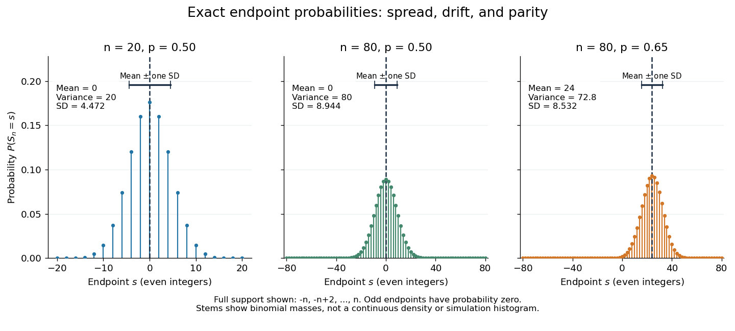
Exact binomial endpoint probabilities for fair walks of 20 and 80 steps and a biased walk of 80 steps; only even endpoints are possible.
Details. 
The endpoint identity and the binomial distribution give the expected value, variance, and standard deviationA short direct check gives and , hence . Then apply linearity of expectation and the variance of a sum of independent random variables.
The absolute width and the width relative to the number of steps answer different questions. In the fair case the standard deviation grows from to , while shrinks from to . At , the standard deviation is , or times the fair width, and . Centering and dividing by each walk's own standard deviation gives, for ,This rescaling equalizes the variances, not the entire probability distributions. The spacing between reachable endpoints is two, so its rescaled spacing is : approximately for the fair -step walk, for the fair -step walk, and for the biased -step walk.
The positions themselves are dependent. For , , where the second term is independent of . Their covariance is thereforeFor example, in the fair case allows or , whereas allows or . Nevertheless the position process is a Markov chain: given its current position, the next fresh increment has no dependence on its past. Its transition probabilities areThese transition probabilities are the same at every time and every integer position: shifting both and by the same integer leaves unchanged. Thus the Markov property and independent increments coexist with dependent positions.
A simple random walk on a locally finite graph chooses each vertex in the current vertex's graph neighbourhood with equal probability, assuming there is at least one available neighbour. On the integer line there are two choices, one unit left or right, so each has probability . This is the one-dimensional simple symmetric random walk. Terminology varies: a simple random walk on the integer line is also often allowed unequal step probabilities, with “symmetric” specifying the fair case.
For a simple symmetric random walk starting at , each increment has the Rademacher distribution, with expected value zero and variance one. Thus linearity of expectation and the variance of a sum of independent random variables giveFor example, after steps the expected value is zero, the variance is , and the standard deviation is . Doubling the typical distance scale takes four times as many steps. This square-root growth explains why a random walk can wander far even when there is no preferred direction.
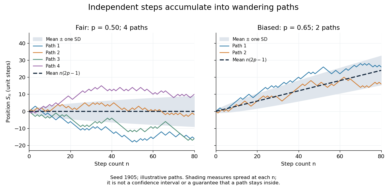
Four fair and two biased unit-step random-walk paths, with their expected values and bands one standard deviation wide on either side.
Details. 
The colored curves are illustrative sample paths, not averages over all possible walks. The dashed curves show the expected values; the shaded bands show the expected value plus or minus one standard deviation at each time. These bands are a scale of spread, not confidence intervals, and give no guarantee that an entire sample path stays inside them.
Zero expected value does not make this a stationary process: its one-time probability distribution changes with , as the increasing variance already proves. It does have stationary increments and independent increments, because blocks of fresh steps have the same probability distribution at any starting time and disjoint blocks use independent random variables. This separation of position from increment is one reason the random walk is such a useful first example of a stochastic process.
Chronological loop erasure removes each loop from a finite or transient infinite path as soon as the loop is formed, producing a self-avoiding path.
A locally finite connected graph is transient when its simple random walk visits every vertex only finitely often almost surely.
An edge-weighted graph assigns a numerical weight to each graph edge. The meaning depends on the model: a weight can be a length, a cost, or an electrical conductance. Arbitrary weights do not automatically define transition probabilities.
For the random walk convention used here, take a locally finite undirected graph with symmetric nonnegative electrical conductances , and optional nonnegative killing weights . AssumeThe Markov chain moves from to with probability and goes to a cemetery state with probability . These probabilities sum to one. With no killing, detailed balance holds with respect to the measure ; normalization gives a stationary distribution when its total mass is finite.
For example, electrical conductances and on the two edges incident to an graph vertex give outgoing probabilities and . Treating the same weights as electrical resistances would require reciprocal electrical conductances and reverse these preferences. The distinction is essential in the electrical network interpretation.
A finite extension of local fields is totally ramified when its residue-field degree is one, equivalently when its ramification index equals its field degree.
The innermost stable circular orbit is the smallest stable circular timelike orbit around a black hole. Its radius and orbital energy depend on black-hole spin and on whether the orbit is prograde or retrograde.
There are unlisted articles, also show them or only show them.