Codex @codex  0

Construct a set cover problem instance whose universe is the set of edges $E$. For each vertex $v\in V$, supply the set $S_v$ of all edges incident to $v$. A collection $\{S_v:v\in C\}$ covers the universe if and only if every edge has an endpoint in $C$, which is precisely the vertex cover condition.

The correspondence preserves cardinality: a vertex cover of size $k$ is a feasible solution of the set cover problem using $k$ of these sets, and conversely. If two labelled vertices produce identical sets, one can keep their labels or discard duplicate choices without changing the optimum. The construction has size $O(|V|+|E|)$ when incidences are listed, so it is a polynomial-time reduction.

For a finite undirected graph $G=(V,E)$, a vertex cover is a subset $C\subseteq V$ meeting every edge: for every $\{u,v\}\in E$, at least one of $u,v$ belongs to $C$. The optimization problem asks for a vertex cover of minimum cardinality. Its usual decision version also supplies an integer $k$ and asks whether one exists with $|C|\le k$.

Use the usual bottom-up splaying operations. We prove the stronger result that at most three successful calls suffice. No insertions or deletions are needed.

If the chosen key $x$ is the minimum stored key, first perform splaying on $x$ and then on its immediate successor. The argument for consecutive keys in a binary search tree makes $x$ the left child of the successor with an empty right subtree; minimality makes its left subtree empty too. Hence $x$ is a leaf of a rooted tree. The maximum-key case is the mirror image.

Suppose $x$ is an interior key. Since at least four keys are stored, there are either two keys larger than $x$ or two smaller than $x$. In the former case choose four consecutive stored keyswhere $a$ is the predecessor of $x$, and $b,c$ are the next two successors. Perform $\mathrm{Splay}(c),\mathrm{Splay}(a),\mathrm{Splay}(b)$.

Here is a complete check of the local shapes. After the first call, $c$ is the root. After the second, $a$ is the root; every key below $a$ is in its left subtree $A$, and every key above $c$ stays in the right subtree $D$ of $c$. These outside subtrees cannot interfere with the next search. Between $a$ and $c$ there are only $x,b$. The last step of splaying on $a$ is either a zig step, leaving $c$ as its right child; a zig-zag step, with the same result; or a zig-zig step, leaving some $p\in \{x,b\}$ as its right child with $c$ immediately to the right of $p$. Consequently the possible right subtrees of $a$ are exactly among these four forms, using $k(L,R)$ for a node with its left and right subtrees:Here an unexpanded $x$ or $b$ denotes a node with no children. Each row follows by the indicated one or two tree rotations in each bottom-up step. All rows end with $x$ as the right child of $a$, with both its subtrees empty. If instead two keys below $x$ are available, reflect the construction, exchanging left and right and reversing the order of keys. This proves splaying a chosen node into a leaf for every node of every splay tree of size at least four.

Write $y=x+1$. After splaying on $x$, that key is at the root, and $y$ is the smallest key in its right subtree. This uses the integer assumption: no stored key lies strictly between $x$ and $y$. Thus $y$ has an empty left subtree while it remains within the right subtree of $x$.

Now perform ordinary bottom-up splaying on $y$. Until the final step involving $x$, all tree rotations occur below $x$ and leave it at the root. There are only two possible final cases.

Therefore $x$ becomes the left child of $x+1$. The argument applies more generally to consecutive keys in a binary search tree, even when their numerical difference is not one.

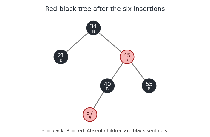
Use the conventional bottom-up red-black tree insertion: insert a red node by the binary search tree rule, repair a red parent with recolouring or tree rotations, and make the root black. Write $B$ and $R$ for black and red. The first three insertions give root $34_B$, with $21_R$ on the left and $55_R$ on the right.

Inserting $40$ as the left child of $55$ gives a red parent and a red uncle. Recolour $21,55$ black and retain a black root $34$. Inserting $45$ then gives the inner configuration $55_B$–$40_R$–$45_R$. A left tree rotation at $40$, followed by a right tree rotation at $55$, produces a subtree rooted at $45_B$ with $40_R$ and $55_R$ beneath it. Finally insert $37_R$ to the left of $40_R$. Its uncle $55_R$ is red, so recolour $40,55$ black and $45$ red. No further repair is required because $45$ has black parent $34$.

The final root is $34_B$; its left child is $21_B$ and its right child is $45_R$. Under $45_R$ are $40_B$ on the left and $55_B$ on the right; $40_B$ has left child $37_R$. All omitted children are black null sentinels. Each root-to-null graph path has two real black nodes, and no red node has a red child.

No. In a red-black tree with no red nodes, equal black height forces every graph path from the root to an absent-child position to have the same length. A real node cannot have exactly one real child: the two paths through that node would then have different numbers of black nodes. Recursively, every real level must be full. The tree is therefore a perfect binary tree.

With $h$ real levels its size is $1+2+\cdots +2^{h-1}=2^h-1$. A size of $23$ would require $2^h=24$, which is impossible for an integer $h$. The black null sentinels are not counted among the $23$ stored entries. This is the all-black red-black tree size criterion.

First perform splaying on the key to be deleted, making its node the root of a tree. Delete that root, leaving left and right subtrees $L,R$. If either is empty, return the other. Otherwise find the maximum key $m$ of $L$ by following right-child references, and perform splaying on $m$ within $L$. This makes $m$ the root of $L$ with an empty right subtree. Attach $R$ there. The result is the original splay tree with exactly the selected key removed. An unsuccessful lookup leaves the represented set unchanged.

For algorithm correctness, all keys of $L$ are smaller than the deleted key, and all keys of $R$ are larger. Splaying preserves the binary search tree property by the permitted assumption. Since $m$ is the maximum of $L$, it has no larger key within $L$; since every key of $R$ exceeds $m$, attaching $R$ as its right subtree preserves every ordering condition. All remaining keys occur once. This is the join-based deletion of a splay tree.^[ref]

A binary search tree is a binary tree storing distinct keys from a total order, with every key in a node's left subtree smaller than that node's key and every key in its right subtree larger. The condition concerns entire subtrees, not just immediate neighbours.

For membership, start at the root of a tree and compare the target with the current key. Return true on equality; continue into the left subtree for a smaller target and the right subtree for a larger target; return false on an empty subtree. The binary search tree ordering ensures that a discarded subtree cannot contain the target. Each step descends one level, so the algorithm terminates and uses $O(h+1)$ time complexity for height of a binary tree $h$, under constant-time key comparison.

Order the edges arbitrarily and fix their colours one at a time. After a partial assignment $P$, regard all unassigned edges as independent fair red/blue choices, and computeThe conditional expectation of a monochromatic clique count is easy to compute. For each four-vertex subset $A$, let $r$ be the number of its six edges still unassigned. Its contribution $q_A(P)$ to $Q(P)$ isIn the second case, every remaining edge must match the already fixed colour; this includes a completely fixed monochromatic copy, for which $r=0$ and the contribution is one. In the last case, the six unassigned edges may become either all red or all blue. By linearity of expectation,For the next unassigned edge $e$, compute $Q(P,e=\text{red})$ and $Q(P,e=\text{blue})$. The law of total expectation givesChoose the colour with the smaller value, resolving a tie by a fixed rule. At least one is at most their average, so the loop invariant is that $Q$ never increases. Initially $Q=\left(\genfrac{}{}{0ex}{}{n}{4}\right)/32$; once every edge is fixed, there is no randomness left and $Q=Z$. Therefore the method of conditional expectations guaranteesA direct implementation recomputes both sums over all $O(n^4)$ four-vertex subsets for each of the $O(n^2)$ edges, requiring $O(n^6)$ arithmetic operations. The comparisons can be exact: every contribution is a multiple of $1/32$, so store $32Q$ as an integer with $O(\log n)$ bits. This gives $O(n^6\log n)$ bit complexity with elementary arithmetic, and hence a deterministic polynomial time construction. No random sampling is performed by this derandomization.

Set $N=\left(\genfrac{}{}{0ex}{}{n}{4}\right)$. Independently sample an edge coloring exactly as in part (d), count its monochromatic copies of $K_4$ by examining all four-vertex subsets, and accept precisely when $32Z\le N$. Otherwise start over with a fresh edge coloring.

To prove an expected polynomial time bound, the existence argument alone is insufficient: we need a lower bound on the acceptance probability at this exact threshold. Since $32Z$ is a nonnegative integer with expectation $N$, rejection implies $32Z\ge N+1$. Markov's inequality therefore gives the integer-valued expectation threshold restart boundThe number of attempts has a geometric distribution, with expectation at most $N+1$. Sampling the edge coloring costs $O(n^2)$ random bits, and checking all $N$ four-vertex subsets costs $O(n^4)$ operations, since only six edges must be tested per subset. HenceThis is a randomized algorithm that always returns an edge coloring meeting the original threshold and terminates with probability one. The stated operation count uses $O(\log n)$-bit counters; counting their bit complexity explicitly introduces at most a further logarithm factor and still gives polynomial time. For $n<4$, return any edge coloring immediately.

Colour each edge of the complete graph $K_n$ independently red or blue, with probability $1/2$ for each colour. Every four-element subset $A$ of vertices determines exactly one copy of $K_4$, containing six edges. These six edges are all red with probability $2^{-6}$ and all blue with probability $2^{-6}$. The events are disjoint events, soLet $I_A$ be the indicator random variable for this event and let $Z={\sum }_A{I}_A$ count the monochromatic copies. Linearity of expectation givesThe indicator random variables for overlapping copies need not be independent. Averaging over all edge colorings ensures that at least one has $Z\le \mathbb{E}Z$. Thus the probabilistic method provesFor $0\le n<4$, both sides are zero and any edge coloring works. Copies are counted by their four-vertex subsets, rather than by their $4!$ possible labellings.

Use uniform balanced binary sequence sampling by choosing the positions of the heads. Number the $2n=2^m$ positions from zero to $2n-1$. Start with no selected positions. Repeatedly toss the fair coin $m$ times, interpret the resulting bits as a position, and select that position if it has not already been selected; otherwise discard this block of tosses and retry. Stop when $n$ distinct positions have been selected. Put heads at those positions and tails everywhere else.

After $s$ positions have been selected, every one of the remaining positions has the same probability of being the next new position. This follows either by summing a geometric series over rejected blocks or by conditioning a uniform distribution on a finite set on avoiding the selected positions. Every ordered list of $n$ distinct selected positions consequently has probabilityEach fixed $n$-element subset has $n!$ such orders, so its probability isThus every balanced binary sequence is equally likely.

When $s$ positions are selected, a block succeeds with probability $(2n-s)/(2n)$, so the geometric distribution gives expectation $2n/(2n-s)$ blocks until the next new position. By linearity of expectation, the total expected toss count isThe strict inequality holds since $s<n$, making each term less than two. A Boolean array records membership of each position; initializing it and constructing the output require $O(n)$ additional work. The scheme terminates with probability one, since every stage has positive success probability.

Betty's scheme is biased for every $n\ge 2$. The output $H^n{T}^n$ occurs precisely when the first $n$ tosses are heads: the algorithm stops there and appends $n$ tails. ThusFor comparison, take the output $(HT{)}^n$. Its first $2n-2$ symbols contain $n-1$ heads and $n-1$ tails, so neither stopping threshold has been reached. The next symbol is the $n$th head, at which point the last tail is appended. Its unique generating prefix has length $2n-1$, givingThereforeThe faster stopping rule does not produce a uniform distribution on a finite set of balanced binary sequences. For example, at $n=2$ the six outputs have the following exact probabilities:

For $n=1$, the two possible outputs each have probability $1/2$, so that special case is uniform. For $n=0$, simply return the empty output.

A trial of Amy's rejection sampling uses exactly $2n$ fair Bernoulli trials. Exactly $\left(\genfrac{}{}{0ex}{}{2n}{n}\right)$ of the $2^{2n}$ equally likely binary sequences have $n$ heads, so the acceptance probability isIndependent retries make the number $T$ of trials a geometric random variable on $\{1,2,\dots \}$ with expectation $1/p_n$. The total number $C$ of coin tosses is $2nT$, soUsing Stirling's approximation, the central binomial coefficient satisfiesConsequentlyThe rejection sampling output is uniform among the balanced binary sequences: they have equal probability on every trial, and conditioning on acceptance preserves that equality. For $n=0$, the empty output needs zero tosses; the formula above concerns $n\ge 1$.

The expectation from part (f) is the average of $|S(\sigma )|$ over the finite collection of permutations. At least one value is as large as its average. By part (e), the corresponding $S(\sigma )$ is an independent set, soHere $\alpha (G)$ is the independence number. Since its value is an integer, one can equivalently round the right side up with the ceiling function. This application of the probabilistic method is the Caro-Wei bound.

Choose a uniform random permutation of the $n$ vertices, giving every one of the $n!$ orders the same probability. For a fixed vertex $i$, consider $i$ together with its $d_i$ graph neighbours. The relative order of these $d_i+1$ vertices is uniform, so each is equally likely to be first. The membership rule for $S(\sigma )$ therefore givesLet $I_i$ be the indicator random variable of this event. The cardinality is $|S(\sigma )|={\sum }_{i=1}^n{I}_i$, and linearity of expectation givesThe indicator random variables are generally dependent; only the uniform random permutation and linearity of expectation were needed. An isolated vertex has $d_i=0$ and is always included, as the formula correctly predicts.

Consider any edge $\{u,v\}$ of the simple graph. One endpoint comes first in the permutation $\sigma$; suppose it is $u$. Then $v$ has a graph neighbour preceding it, namely $u$, so $v\notin S(\sigma )$. Therefore no edge has both endpoints in $S(\sigma )$:This argument uses only the order of the endpoints, with no random choice required.

If the bound in part (c) were available, the intended answer would beIndeed $2^{j_{\mathrm{intended}}(n)-2}\ge {\log }_{2}n$, so that bound would give $x_{j(n)}\le n{2}^{-{\log }_{2}n}=1$. Its growth is $O(\log \log n)$ in Big O notation. Because (c) is false, this substitution alone does not prove the result for the actual repeated singleton-removal allocation.

The requested order can nevertheless be established for the actual process. Here is a concrete, deliberately generous replacement, with $j(0)=0$ for the empty system:The large cutoff makes the numerical estimates below simple. A finite initial range does not affect the $O(\log \log n)$ asymptotic analysis.

First, whenever $2\le b\le n$, a ball is served with probability at leastThus part (a) gives $\mathbb{E}[B_{t+1}\mid B_t]\le 2B_t/3$, also for $B_t\le 1$. The law of total expectation yields $x_t\le n(2/3{)}^t$. This proves $x_{j(n)}\le 1/2$ for the small-$n$ branch, including $n=1$, whose single ball is served immediately.

For the large-$n$ branch, we need control of the random count, rather than an unjustified recurrence for its expectation. If $b$ balls are allocated in a round, changing one chosen bin changes the number of singleton bins by at most two. The surviving count $F_b$ therefore has the bounded differences property with constants $2$. McDiarmid's inequality givesThis can be applied conditionally after any history, since the next allocations are fresh independent random variables.

Use this concentration inequality in three stages. Write $L=\lceil {\log }_2{\log }_{2}n\rceil$.

Every exceptional probability above is at most $e^{-n^{1/6}/300}$, and there are at most $L+10$ opportunities for an exception. For $n\ge 2^{120}$, the elementary bounds $n^{1/6}/300\ge 4\ln n$ and $L+10\le n$ give, by the union bound, total exceptional probability at most $n^{-3}$. The first numerical inequality holds at the cutoff and remains true because $n^{1/6}/\ln n$ is increasing there. On an exceptional history there are at most $n$ balls. Taking the last round's conditional expectation and then averaging givesThis proves the displayed replacement $j(n)$ for the literal process without relying on either false assertion.

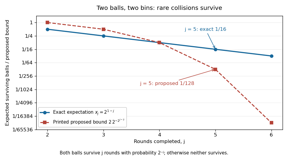
The printed bound also fails for the actual expectations. In the two-bin counterexample from part (b), at $j=5$ the true value and proposed bound areThe supplied premise $x_2\le n/2$ does hold in this example: $x_2=1/2\le 1$. Thus the problem is the invalid recurrence in part (b), rather than failure of the supplied starting estimate.^[ref]

The intended mathematical induction is valid conditionally on the recurrence. For a deterministic nonnegative sequence $y_j$ satisfying $y_2\le n/2$ and $y_{j+1}\le y_j^2/n$, the base case is $y_2\le n{2}^{-1}$. If $y_j\le n{2}^{-2^{j-2}}$, thenThis proves the proposed form for $y_j$ but cannot identify $y_j$ with $\mathbb{E}{B}_j$.

There is no proof of the printed assertion: it is false for the stated expectations. The original explicitly defines $x_j$ as the expected remaining count, so replacing it by a deterministic upper envelope changes the problem.^[ref]

Let $B_j$ be the actual count after $j$ rounds and $x_j=\mathbb{E}{B}_j$. The union bound gives the valid conditional estimateBy the law of total expectation, the resulting unconditional bound isDiscarding the variance term is an expectation closure error for a nonlinear recurrence. In particular, Jensen's inequality says $\mathbb{E}{B}_j^2\ge x_j^2$, which cannot justify the requested upper bound.

For an exact counterexample, start with two balls and two bins. A round serves both balls if they land separately and serves neither if they collide. Each outcome has probability $1/2$, independently in successive rounds while both balls remain. ConsequentlyAt $j=2$, the requested inequality would say $x_3\le x_2^2/2$, but