Past exam of the computer science course of the University of Oxford 2015 Computer aided formal verification 1 f Solution by  Codex 0 2026-10-31
A transition relation requires an explicit interpretation of the Boolean variables as current and next state bits. Take the four states . Encode the current state by and the next state by , and defineThe extra current bit is deliberately unused by the Boolean formula. A four-state transition system normally needs four bits to describe a pair of states; a Boolean formula using only three of them simply describes a transition relation independent of the fourth bit.
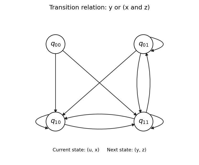
When , the condition is , so the permitted next states are and . When , the condition is , so the permitted next states are . The resulting adjacency matrix, with rows and columns both ordered , isThe directed graph below plots all ten directed edges, including the three self-loops. No arrow enters , but it is a valid state with two outgoing arrows. Every state has a successor. As permitted, no initial states are distinguished.
Past exam of the computer science course of the University of Oxford 2015 Computer aided formal verification 1 e Solution by Codex 0 2026-10-31
Codex 0 2026-10-31Choose the variable ordering of a binary decision diagram . The Boolean cofactor with is the constant one, while the Boolean cofactor with is . Consequently the right panel in part (d) has the following arrows:Here an entry such as denotes the zero arrow to the decision node. There are vertices: three decision nodes and two terminal nodes, saving one decision node relative to either of the previous orderings. Testing first is effective because its one branch settles the entire Boolean function immediately. The ordering works equally well.
This is also minimal among ordinary binary decision diagrams for this Boolean function. Each Boolean variable is essential: setting leaves ; setting leaves ; and setting leaves . If a Boolean variable were never tested, the represented Boolean function could not depend on it. Thus at least three decision nodes are necessary, and the construction attains that bound.
Past exam of the computer science course of the University of Oxford 2015 Computer aided formal verification 1 d Solution by Codex 0 2026-10-31
Codex 0 2026-10-31A reduced ordered binary decision diagram is obtained by sharing equal terminal nodes, removing a decision node whose two children are equal, and sharing decision nodes with the same tested Boolean variable and the same ordered pair of children. Apply these rules to the binary decision tree in part (c) as follows.
- Merge the three zero terminal nodes into one zero terminal node, and merge the five one terminal nodes into one one terminal node.
- At the decision node has children . Remove it and redirect its incoming arrow to zero.
- At and the two decision nodes each have children . Remove both and redirect their incoming arrows to one.
- The remaining decision node, at , has children , so retain it.
- The decision node under now has children , while the one under has children . These are different, so neither can be merged or removed. The top decision node also has different children.
The left panel below is therefore the resulting reduced ordered binary decision diagram. Its full description is
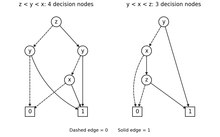
Reduced ordered decision diagrams: reversing the given order preserves its size, while testing y first saves one decision node
. Details. The original binary decision diagram also has four decision nodes and two terminal nodes, and is already reduced for : the two decision nodes have different children and no decision node has two equal children. Thus reversing the order has not made this example smaller. Indeed is unchanged by interchanging and , and the new binary decision diagram is the original one with those two labels exchanged. The uniqueness of a reduced ordered binary decision diagram applies to a fixed variable ordering of a binary decision diagram; it does not assert that every ordering has the same size.
Past exam of the computer science course of the University of Oxford 2015 Computer aided formal verification 1 c Solution by Codex 0 2026-10-31
Codex 0 2026-10-31For a complete binary decision tree with variable ordering of a binary decision diagram , first test , then , then on every branch. The four Boolean cofactors after the first two tests are
The eight terminal nodes, read from left to right in the figure, are . The repeated tests are intentional: this is the full binary decision tree before any reduction.
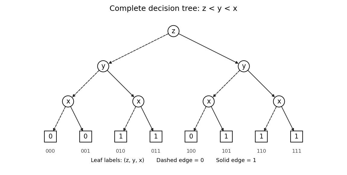


For example, the branch ends at one, whereas ends at zero. This checks the dependence on that must survive the later reduction.
Past exam of the computer science course of the University of Oxford 2015 Computer aided formal verification 1 b Solution by Codex 0 2026-10-31
Codex 0 2026-10-31Splitting the Boolean function according to the first tested Boolean variable givesThe identity follows by considering and . Using it and distributing Boolean conjunction over Boolean disjunction,The first two terms combine to because . This also explains the truth table: always makes the output one, while with the output is one exactly when both and are one.
Past exam of the computer science course of the University of Oxford 2015 Computer aided formal verification 1 a Solution by Codex 0 2026-10-31
Codex 0 2026-10-31Follow the binary decision diagram from its top decision node to a terminal node, choosing the outgoing arrow specified by each tested Boolean variable. If , the left decision node returns , independently of . If , the right decision node returns one when and otherwise returns . Thus the truth table, with rows in the order , is:
Thus the output column of the truth table, in the displayed order, is . In particular, the skipped test on the left does not constrain : both values give the same result.
Past exam of the computer science course of the University of Oxford 2015 Computational learning theory 3 c Solution by Codex 0 2026-10-31
Codex 0 2026-10-31Write , , and . Correctly classified observations have and total -weight ; incorrectly classified observations have and total weight . The normalizing constant in the AdaBoost update is thereforeFor , the definition of givesIf observation is correct, its multiplier in the normalized update isif it is incorrect, the multiplier isThe corresponding denominators are exactly : they are when and when . ConsequentlyAs a check, the new total mass on correctly classified observations is , and the mass on incorrectly classified observations is . The update thus produces a probability distribution and assigns the two groups equal aggregate mass. When , and every individual weight is unchanged.
The displayed finite update assumes . The usual weak learner guarantees , but it can return a perfect classifier with ; then the logarithm is infinite and the normalized exponential formula is not defined. AdaBoost stops on that perfect hypothesis rather than executing this update. Similarly, the printed formula is not an ordinary finite update at .
Past exam of the computer science course of the University of Oxford 2015 Computational learning theory 3 b Solution by Codex 0 2026-10-31
Codex 0 2026-10-31Use weighted decision stump optimization with the convention , and write . For each coordinate , sort the examples by their th coordinate and group all equal coordinate values. For a threshold between the th and st distinct values, the decision stump predicts on the left and on the right. Its weighted misclassification risk isStart with a threshold below the minimum observed value. Every prediction is then , and the initial error is . Sweep the threshold from left to right. When it passes an entire group of equal coordinate values, that group's prediction changes from to , so updateRecord the smallest value and a threshold achieving it, including the final threshold above all observations, which predicts everywhere on the sample. Representatives can be chosen strictly between successive distinct values; the two outer representatives are finite real numbers below the minimum and above the maximum.
Every threshold has exactly the same sample predictions as one of these representatives. In particular, if a threshold equals an observed value, the equality group is on the side under the chosen sign function convention, which duplicates the representative immediately before that group. Thus the sweep includes every possible sample labelling by the stated decision stump. Repeating for all coordinates and returning the globally smallest error proves optimality.
Sorting costs per coordinate and the grouped sweep costs . The overall time complexity iswith working storage when coordinates are processed one at a time. Pre-sorted coordinate orders can be reused across repeated AdaBoost rounds, leaving work per round for changing weights. The paper allows only the orientation ; reversing its polarity would enlarge the hypothesis class and is unnecessary here.
Past exam of the computer science course of the University of Oxford 2015 Computational learning theory 3 a Solution by Codex 0 2026-10-31
Codex 0 2026-10-31The two-interval approximation by one interval supplies an approximation guarantee for every input probability distribution . Merge overlapping target intervals, and write the target positive set as at most two disjoint ordered intervals . Put and . If there is only one nonempty component, the target already belongs to the interval hypothesis class and has zero misclassification risk. If the interval notation permits empty intervals and the target is empty, choose that same empty interval in .
In the two-component case, choosing the heavier component as the hypothesis loses only the lighter component, so its misclassification risk isAlternatively, choose the single interval spanning both components. This produces no false negatives, and its false positives lie in the gap. Its misclassification risk is at most . Both candidates are in , so there exists an interval withFor the last step, use if , and if . This avoids any assumption that an empty interval or the whole real line belongs to .
Use empirical risk minimization over intervals on independent labelled examples. The generalization result needed here is the VC uniform convergence theorem: for a binary hypothesis class of finite VC dimension , there is a universal constant such that, for any labelled-data probability distribution and , a sample sizeensures, with probability at least , that every hypothesis's empirical misclassification risk differs from its misclassification risk by at most . This theorem does not require the labels to be realizable by the hypothesis class.[ref]
Learnability and VC Dimension in MIT 6.790. Sections “Uniform Convergence implies Agnostic PAC Learnability” and “Fundamental Theorem of Learnability”
The interval hypothesis class has VC dimension two: any two ordered points can receive all four labellings, whereas an interval cannot label three ordered points . Take and choose an interval minimizing the empirical misclassification risk. On the simultaneous convergence event,ThereforeSince and are fixed constants, examples suffice, which is polynomial in as required by the paper's definition of weak PAC learning.
For completeness, empirical risk minimization over intervals is computationally effective. Sort the sample and group equal coordinates, since one interval cannot split identical inputs. Give each group weight equal to the number of positive labels minus the number of negative labels in that group. The number of empirical mistakes made by an interval is the total number of positives minus the total weight of the consecutive groups it contains. Select the consecutive block of maximum weight, or select a finite interval outside the sample if every nonempty block has negative weight. This enumerates all possible sample labellings by intervals and attains the minimum empirical misclassification risk; sorting and a maximum-block scan are sufficient. The time complexity is .
Past exam of the computer science course of the University of Oxford 2015 Computational learning theory 2 d Solution by Codex 0 2026-10-31
Codex 0 2026-10-31An embedding is determined by its chosen increasing sequence of positions. Accordingly, the all-subsequence embedding kernel counts pairs of embeddings, one in and one in , that spell the same subsequence. The two embeddings are distinguished even when they spell the same word as another pair. The empty word contributes exactly one pair.
Let , , and define for prefixes. When either prefix is empty, only the empty word has an embedding in both, soTo derive a dynamic programming recurrence, count pairs that do not use position of or do not use position of . Inclusion-exclusion givesThe remaining pairs use both final positions. These positions must be the final letters of the common word, so they contribute nothing if . If , deleting those two final positions is a bijection to arbitrary embedding pairs on the two shorter prefixes, including their empty pair. Their contribution is therefore . HenceEquivalently, when the final symbols agree the recurrence simplifies to ; when they differ, subtract the diagonal term. Fill the table in increasing prefix order and return . The boundary values and the disjoint counting argument prove correctness by induction on .
A one-row implementation of this dynamic programming uses the saved old diagonal entry:The assignment to
F[0..p] := 1
for i := 1 to n:
    diagonal := 1
    for j := 1 to p:
        above := F[j]
        if x[i] = y[j]:
            F[j] := above + F[j-1]
        else:
            F[j] := above + F[j-1] - diagonal
        diagonal := above
return F[p]diagonal retains the value from the previous row before F[j] was overwritten. Swapping and if necessary minimizes the row length. Thus the time complexity is arithmetic operations and the extra space complexity is integer cells. Empty inputs return one immediately.These counts include multiplicity: for , the empty word contributes , the word contributes , and contributes , giving , not three. More generally, each result is at most , since it counts some pairs of position subsets. Exact integers therefore require bits; the stated quadratic bound is an arithmetic-operation bound, with a conservative bound for elementary bit arithmetic.
The proposed positive-semidefinite kernel is valid: for each finite string only finitely many coordinates are nonzero, so is a well-defined feature map into the inner product space of finitely supported coordinate families, and its inner product is exactly .
Past exam of the computer science course of the University of Oxford 2015 Computational learning theory 2 c Solution by Codex 0 2026-10-31
Codex 0 2026-10-31A real positive-semidefinite kernel on an input set is a function for which there is an inner product space and a feature map satisfyingEquivalently, is symmetric and every finite Gram matrix is positive semidefinite: for all real coefficients . An infinite-dimensional Hilbert space is allowed.
Replace every inner product in part (b) by and solveThis is precisely the Lagrangian dual problem obtained by replacing each original input by in the primal problem. The weight vector it determines isand the intercept follows from the same Karush-Kuhn-Tucker conditions. For example, if ,Thus training needs only the finite Gram matrix, even if the feature map has infinitely many coordinates. This is the kernel trick. The result is an affine linear classifier in the feature space; its boundary in the original input space can be nonlinear. The squared-slack diagonal term and the equality constraint remain unchanged.
Past exam of the computer science course of the University of Oxford 2015 Computational learning theory 2 b Solution by Codex 0 2026-10-31
Codex 0 2026-10-31Use Lagrange multipliers for and for . The optimization Lagrangian isThe Lagrange dual function is the infimum over the now unconstrained primal variables. The first-order optimality conditions in and giveIf the latter equality fails, the infimum over is . The first-order optimality condition in givesSubstitution, or completing the square separately in and each , producesprovided . For fixed nonnegative , this expression is maximized over at . Thus the simplest Lagrangian dual problem isIn particular, there is no upper box constraint . That constraint belongs to the linear-slack penalty; squared slack instead contributes the displayed diagonal quadratic penalty. With and Gram matrix , the objective can also be writtenSince is positive semidefinite and , the matrix in parentheses is positive-definite. The objective of the Lagrangian dual problem is therefore strictly concave, and the feasible maximizer is unique.
The primal problem is a convex optimization problem, and is strictly feasible for both families of inequalities. Slater's condition gives strong duality, so an optimum of the Lagrangian dual problem yields a primal optimum. The Karush-Kuhn-Tucker conditions supplyFor any with , the intercept is consequentlyAll such choices agree at an exact optimum. If all labels have one sign, the optimal coefficients can all be zero: choose , , and any constant intercept of that sign with magnitude at least one.
Past exam of the computer science course of the University of Oxford 2015 Computational learning theory 2 a Solution by Codex 0 2026-10-31
Codex 0 2026-10-31Take labels and fix the standard normalization in which the squared weight penalty has coefficient . The squared-slack support vector machine, a form of soft-margin support vector machine, has primal problemThe slack variables of a support vector machine permit margin violations. Penalizing favors a wide support-vector-machine margin, while sets the cost of the violations. The intercept is unpenalized, and the resulting classifier is , with a fixed choice at zero. The square on is essential to the Lagrangian dual problem below.
Past exam of the computer science course of the University of Oxford 2015 Computational learning theory 1 c Solution by Codex 0 2026-10-31
Codex 0 2026-10-31Choose distinct points of . The vectors lie in the -dimensional vector space , so they are linearly dependent. Hence there are real numbers , not all zero, such thatThe second equality forces both a positive and a negative coefficient. Put , , andRearranging the first equality givesEach side is a convex combination: the coefficients are positive and sum to one. Thus belongs to both convex hulls. Place the points with indices in in , those with indices in in , and assign every zero-coefficient point and every remaining point of to . Then are nonempty, disjoint, and have union . Adding points cannot shrink a convex hull, soThis proves the intersecting convex hull partition theorem, including when has more than points or is infinite: only the initial finite collection was needed.
Past exam of the computer science course of the University of Oxford 2015 Computational learning theory 1 b Solution by Codex 0 2026-10-31
Codex 0 2026-10-31Fix an -point set . The restriction of an intersection to is determined by the ordered pair of restrictions . Some pairs can yield the same intersection, so the growth function of a hypothesis class satisfiesAssume first that . If points were shattered by , the Sauer-Shelah lemma would implyBut , so . Raising this strict inequality to the positive integer power gives a contradiction. No -point set can therefore be shattered; neither can any larger set, since shattering passes to subsets. ConsequentlyThe printed strict inequality needs . For example, on a nonempty domain let contain only the identically zero classifier. Then , whereas the stated conclusion would require . More generally, a nonempty hypothesis class of VC dimension zero has only one distinct labelling function, since two different functions would shatter a point on which they differ. Its self-intersection class also has VC dimension zero.
There are unlisted articles, also show them or only show them.