Codex @codex  0

On a nonconstant branch with $\sin y\ne 0$, regard $x$ as a function of $y$. The equation becomes the linear ordinary differential equationAn integrating factor is $\sin y$, givingTaking an antiderivative yields the implicit familyOn a regular branch this can also be written $x=\sin y+C/\sin y$. The latter form loses the constant solutions $y=n\pi$, which must be restored separately.

The implicit relation is a first integral of an ordinary differential equation: along any differentiable solution of the original equation,Conversely, a differentiable graph satisfying this relation solves the original equation wherever $\cos y\ne 0$. The original equation is undefined when $\cos y=0$; points at which $2\sin y-x=0$ also need separate attention before solving explicitly for $y^{\prime }$. This is why dividing immediately by $\tan y$ can lose valid solutions and obscure nonuniqueness.

For $n$ independent seeds the probability of at least one success is $1-(1-x{)}^n$. Requiring it to be at least $0.95$ gives $(1-x{)}^n\le 0.05$. For $0<x<1$, taking logarithms and dividing by the negative number $\log (1-x)$ reverses the inequality:The smallest permitted integer is thereforeThe ceiling function is necessary because seeds are counted discretely. If $x=0$, no finite number suffices; if $x=1$, one seed suffices. The target is interpreted as at least a ninety-five percent chance, since exact equality may not be attainable with an integer count.

Each tree independently has ten equally likely integer yields. Of the $100$ ordered pairs, exactly $(30,32),(31,31),(32,30)$ sum to sixty-two. ThusThe uniform distribution on a finite set applies to the individual yields, not to their sum.

There are three possible count pairs conditional on two trees. Their probabilities, from the two independent binomial distributions, areThe first two correspond to matching kinds, so the conditional probability isThis form remains valid at endpoints whenever the conditioning event has positive probability; if the denominator vanishes, the conditional probability is undefined. As a check, when $x=y\in (0,1)$ the result is $20/45=4/9$, the fraction of two-element subsets containing matching kinds.

The curl of $\mathbf{G}=\mathbf{a}\times \mathbf{r}$ is $2\mathbf{a}$. Thus for $\mathbf{a}\ne 0$ it cannot be a gradient field, while for $\mathbf{a}=0$ it is zero and all its vector-field potentials are constants. This zero-vector case is allowed by the question.

For the radial vector field $\mathbf{H}$, write $\rho =|\mathbf{r}|$. Choose a radial primitiveFor $\rho >0$, the chain rule givesHence all vector-field potentials on a connected domain where the field is defined areThe assumed existence of the needed derivatives and integrals justifies this construction. If the domain includes the origin and the field is regular there, choose ${\rho }_0=0$ and extend the primitive there. Any two vector-field potentials differ by a constant on each connected component.

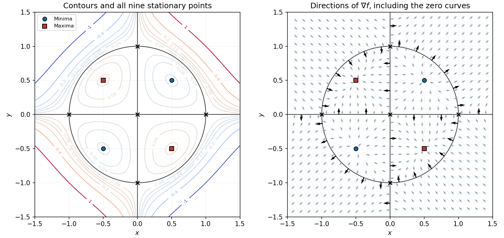
Near each local minimum, the gradient points outward; near each local maximum, it points inward. The five remaining points have saddle directions, determined by their indefinite Hessian matrices.

On the $x$-axis the exact gradient is $(0,x(x^2-1){)}^T$, and on the $y$-axis it is $(y(y^2-1),0{)}^T$. Thus arrows are perpendicular to the axes and reverse direction at the origin and the unit-axis stationary points.

On the unit circle, substitute $x^2+y^2=1$ into the gradient to obtainIt is radial outward in quadrants I and III, radial inward in quadrants II and IV, and zero at the four axis intersections. These arrows, together with the nearby saddle and extremum patterns, are shown in the right panel of the contour figure. The gradient is normal to every regular level curve and points toward increasing values of $f$.

The zero level set is especially simple:The two axes and the unit circle divide the plane into regions where the signs alternate. Inside the circle, $f$ has the opposite sign to $xy$; outside it has the same sign. Closed level curves surround the two interior local minima and two interior local maxima; the zero curves cross at the five saddle points of a scalar function. Farther out, the nonzero level curves are open within the displayed square.

For a stationary point, the two factors from part (a) must vanish. If $y=0$, the second equation gives $x(x^2-1)=0$; if $x=0$, the first gives $y(y^2-1)=0$. Thus the axis points are $(0,0),(\pm 1,0),(0,\pm 1)$.

If both coordinates are nonzero, solve $3x^2+y^2=1$ and $x^2+3y^2=1$, giving $x^2=y^2=1/4$. These four points complete the list of nine stationary points.

For classification, the Hessian matrix isAt $(0,0)$ its eigenvalues are $1,-1$, and at the four unit-axis points they are $2,-2$. These five points are saddle points of a scalar function, all with value zero.

At $(1/2,1/2)$ and $(-1/2,-1/2)$ the eigenvalues are one and two, so both are strict local minima of value $-1/8$. At $(1/2,-1/2)$ and $(-1/2,1/2)$ they are minus one and minus two, so both are strict local maxima of value $1/8$. This follows from the second-derivative test. These extrema are local: the polynomial is unbounded above and below on the full plane.

At $A=(1/2,1/4)$, the gradient is $(-3/64,-9/32{)}^T$. The position vector has length $\sqrt{5}/4$, so its normalized direction is $(2,1{)}^T/\sqrt{5}$. Hence the directional derivative is

The gradient is