An invocation made by a recursive procedure of itself, directly or through another procedure. Each invocation has its own arguments and local variables; a returning invocation supplies an output to its caller.
A case answered without further recursive calls. Complete base cases are one part of an algorithm termination argument; the other cases must progress in a well-founded relation.
A base case and a decreasing natural number measure work together. Check that every invocation satisfies its precondition, each base case finishes with the correct output, and every other invocation makes finitely many recursive calls with strictly smaller measure. All local work must also terminate. By well-founded induction, the children finish, so their caller finishes; if their answers are correct and the combination rule preserves the postcondition, the caller is correct too. This proves total correctness, not just correctness conditional on return.
Strict decrease without a lower bound is insufficient: subtracting one forever from a negative integer never reaches zero. Even a positive real-valued measure can decrease indefinitely, as shows. A well-founded relation rules out that descent. In structural recursion, a proper child subtree of a finite binary tree supplies progress without numeric arguments. The proof obligation is the relation between parent and child instances, together with terminating local work and complete base cases.
Keep an array unchanged, and sum entries in the half-open integer interval of array indices . The precondition requires integers and exact, terminating integer addition. An empty range returns the empty sum zero; a one-entry range returns that entry. Every longer range splits at its middle array index:For the original array , call . The left half returns , the right half returns , and the original invocation returns . The right half's left endpoint increases from zero to two: what decreases is range length , not every argument. Negative entries affect the answer but do not affect algorithm termination.
S(A, l, r):
    require integer indices with 0 <= l <= r <= length(A)
    size = r - l
    if size == 0:
        return 0
    if size == 1:
        return A[l]
    middle = l + floor(size / 2)
    left_sum = S(A, l, middle)
    right_sum = S(A, middle, r)
    return left_sum + right_sum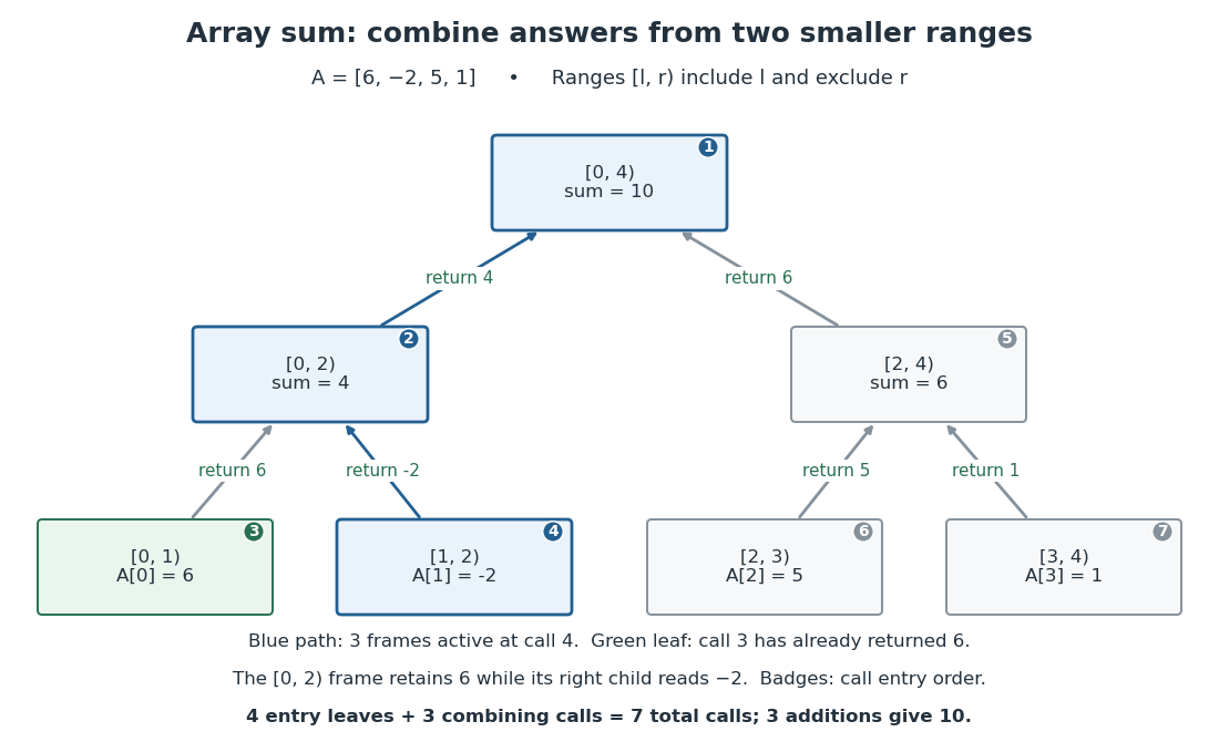
Seven calls compute an array sum with only three frames active at once
. Original binary tree of invocations for , with integer intervals labeling ranges and upward arrows labeling returned sums. Small numbers give the order in which invocations begin when the left child runs first. The highlighted graph path contains the three active stack frames while the entry is read; the result from the completed left sibling is retained by its parent. Details.
For range length , the children have lengths and , both positive and strictly less than . The floor function chooses the split; the ceiling function gives the other length. Algorithm termination follows by this natural number measure. For algorithm correctness, apply mathematical induction on : the two base cases return the specified sum; for a larger range, the two disjoint child ranges cover every original array index exactly once, so addition of their correct sums gives the required sum.
For , the invocation tree is a full binary tree with leaves, one per array entry. If is its number of nonleaf vertices, counting edges gives , so . Thus the total invocation count is , and there are combining additions. Here gives seven calls and three combining additions. For , there is one call and no combining addition; for , there is also one call and no combining addition, but no entry leaf, so the formula does not apply.
The call stack holds the active branch, rather than the entire invocation tree. Execute the left child completely before the right child, retaining the left result in the parent stack frame. The maximum number of active stack frames is for , and one for . Balanced splitting therefore needs frames for , compared with the frames of the factorial recursive process. Assuming constant-cost array access, index operations and addition, its time complexity is and its auxiliary space complexity is machine words for , excluding the stored input. Pass the same array with different endpoints, rather than copying slices. These bounds require all stored indices and partial sums to fit in a constant number of machine words; exact unbounded integer addition and storage require a separate bit cost analysis.
For a natural number , the factorial satisfies and for . The following description includes the zero base case explicitly; a negative or nonintegral input is outside its precondition:For , the arguments on descent are . Each positive-argument invocation postpones one multiplication until its recursive call returns. At the deepest point, the call stack has five stack frames: four suspended callers and the active zero base case. The invocation at zero returns to the invocation at one, rather than finishing the entire computation. Returns then giveA stack frame retains the caller's argument and where to resume. When the invocation at three receives , it uses its own , obtains , and returns that value to the invocation at four. The recursive calls share a definition, but their local variables belong to separate invocations.
F(n):
    require n is an integer and n >= 0
    if n == 0:
        return 1
    child_result = F(n - 1)
    return n * child_result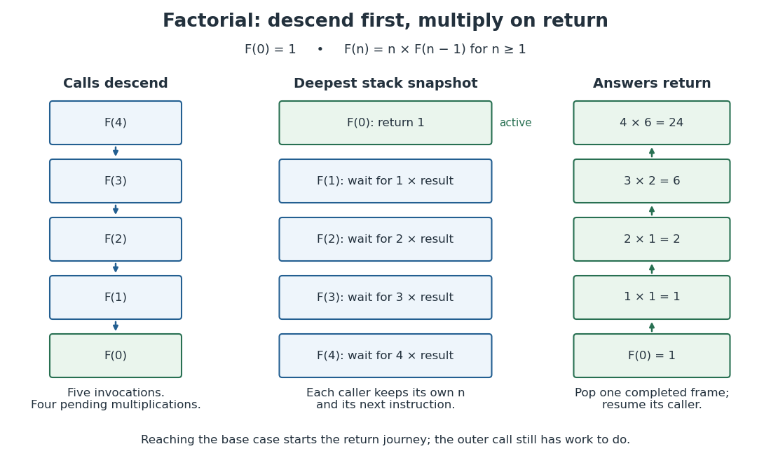

The natural number measure decreases by one on every recursive call, so algorithm termination follows. For algorithm correctness, use mathematical induction: the zero base case returns ; assuming the child's answer is , the caller returns . This also explains why keeping the caller's matters.
There are exactly invocations and multiplications, including one invocation and no multiplications when . Ordinary execution of this recursive process uses at most active stack frames, hence frames for in Big O notation. If each test, call, subtraction and multiplication is counted as constant cost, its time complexity is . That is an arithmetic-operation model: exact arbitrary-length integer multiplication has growing cost, and neither the factorial output nor every stack frame's numeric contents occupies a universally fixed number of bits.
A computation that retains pending operations while further calls run, then completes those operations as results return. A recursive procedure can instead describe an iterative process: passing an updated accumulator onward may leave no arithmetic pending. Avoiding growing call stack storage in that case depends on the implementation. A fixed number of variables also does not imply fixed storage in bits when their integer values grow.[ref]
Structure and Interpretation of Computer Programs by Harold Abelson and others. Structure and Interpretation of Computer Programs, second edition, §1.2.1: deferred operations, state variables, and implementation dependence of space use; bit-storage qualification added here
A procedure whose definition invokes itself directly or indirectly. This is a property of its programming language syntax. It does not determine whether execution accumulates unfinished operations.[ref]
Structure and Interpretation of Computer Programs by Harold Abelson and others. Structure and Interpretation of Computer Programs, second edition, §1.2.1: paragraph beginning “In contrasting iteration and recursion”
Random: Probability, Mathematical Statistics, Stochastic Processes by Kyle Siegrist The Arcsine Distribution by  Codex 0 2026-10-18
Section of Random: Probability, Mathematical Statistics, Stochastic Processes by Kyle Siegrist by Kyle Siegrist. No separate section byline or publication date is established.
Online text: www.randomservices.org/random/special/Arcsine.html
Random: Probability, Mathematical Statistics, Stochastic Processes by Kyle Siegrist The Geometric Distribution by Codex 0 2026-10-18
Codex 0 2026-10-18Section of Random: Probability, Mathematical Statistics, Stochastic Processes by Kyle Siegrist, authored by Kyle Siegrist. Random Services hosts the text. No separately credited section author or publication or revision date is established.
Cited passages: Basic Theory, Definitions; Distribution Functions and the Memoryless Property; Moments.
Random: Probability, Mathematical Statistics, Stochastic Processes by Kyle Siegrist The Pareto Distribution by Codex 0 2026-10-18
Codex 0 2026-10-18Section of Random: Probability, Mathematical Statistics, Stochastic Processes by Kyle Siegrist. Whole-textbook author: Kyle Siegrist; no separate chapter byline is established. Random Services hosts the online text. No publication or revision date is established.
Online text: www.randomservices.org/random/special/Pareto.html
Cited passages: The General Pareto Distribution, Distribution Functions and Moments; Related Distributions, right-tail conditioning and exponential transformation. The section’s parameters must be matched to the shape and minimum conventions used in each application.
For a uniform solid sphere of radius , the squared radius of gyration about its centre is the mass-weighted mean of :Thus its volume is , about . A nonuniform object or a different shape need not obey this conversion. This distinction matters when estimating molecular number density from scattering measurements of a radius of gyration.
Marie Curie's thesis describes powdered material on the lower plate of a capacitor, biased by a battery. Radiation made the intervening air conduct. The upper plate connected to an electrometer and a loaded piezoelectric crystal of quartz. Adjusting the load supplied a known compensating electric charge while keeping the electrometer at zero; charge divided by elapsed time determined the electric current. Voltage scans identified a collection plateau. Contact potentials affected weak-field readings; excessively strong fields could instead introduce additional ionization. Fixed geometry and plateau operation made comparisons meaningful.[ref]
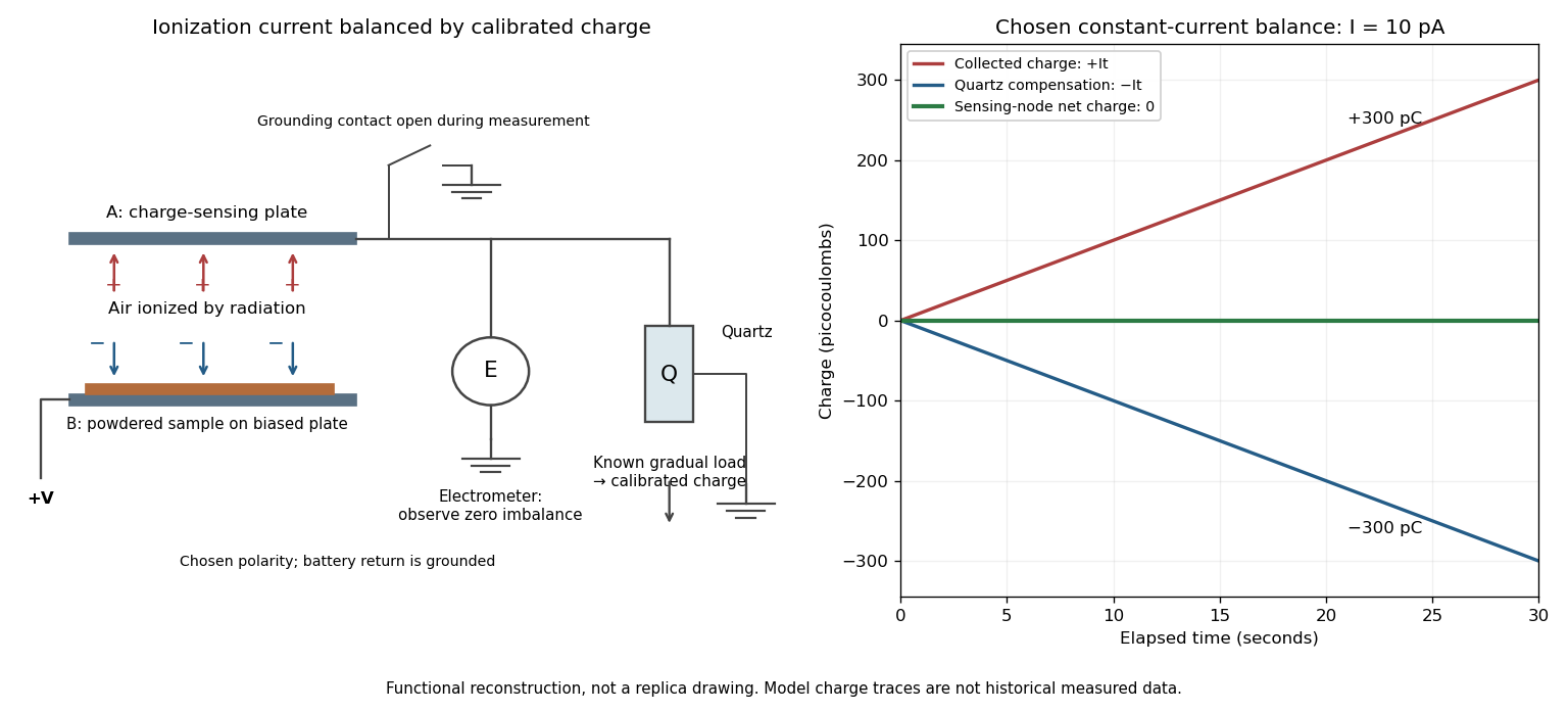

The null method turns a weak signal into a balance against a known quantity. In the diagram's chosen constant-current model, for givesSupplying over the same interval leaves zero net electric charge at the sensing node. The electrometer detects imbalance; the compensating-charge calibration supplies the numerical measurement.
This electric current measures collected charge produced by ionization. Converting it to becquerels additionally requires the energy deposition and charge-collection response per transformation. The apparatus can compare preparations without already possessing that complete source-to-signal calibration.
In his 2 March 1896 report, Henri Becquerel described uranium salt crystals acting on a photographic plate through opaque wrapping. A copper cross weakened the exposure behind it. Plates prepared during intermittent sunshine were left in a drawer and developed on 1 March; unexpectedly strong images prompted deliberate dark tests. He placed a plate and crystals inside two opaque boxes in a drawer; one crystal was separated from the emulsion by glass. After five hours, both produced images. The separation tested transmission without direct chemical contact.[ref]
The result challenged a dependence on immediate illumination. Henri Becquerel still considered long-lasting invisible phosphorescence a possibility, and explicitly withheld a final explanation. The photographic readout established an effect through intervening material; it did not count nuclear transformations or measure a nuclear decay constant.[ref]
Sur les radiations invisibles émises par les corps phosphorescents by Henri Becquerel. Final two paragraphs: tentative invisible-phosphorescence hypothesis and limits of the inference
With parent atomic nuclei present, the conditional expected number of transformations in a short interval is approximately . The corresponding radioactive activity is . Averaging over the finite-population radioactive decay model gives . Its unit is the becquerel.[ref]
10.3 Radioactive Decay. University Physics Volume 3 by Samuel J. Ling and others; Equations 10.17–10.20 and the following becquerel definition
For a finite counting interval, depletion matters. Suppose each transformation is recorded independently with detection efficiency , with at most one count per transformation and no background. The expected value of the count between and isOnly when does this become approximately . A count rate therefore needs a detector model before it can be interpreted as the source's radioactive activity.
Take independently decaying atomic nuclei, each with lifetime drawn from an exponential distribution of rate . With no replenishment, the survivor count isEach indicator variable has success probability , so the binomial distribution givesThe smooth population law is the expected value , satisfying . One realization instead loses whole atomic nuclei at discrete times. An observed count above the smooth curve need not contradict the mathematical model.
For an original chosen example, let and half-life . Then . After , the survival probability is , givingThe standard deviation describes variation between repeated populations governed by these assumptions. It is not an uncertainty interval for a noiseless deterministic curve.
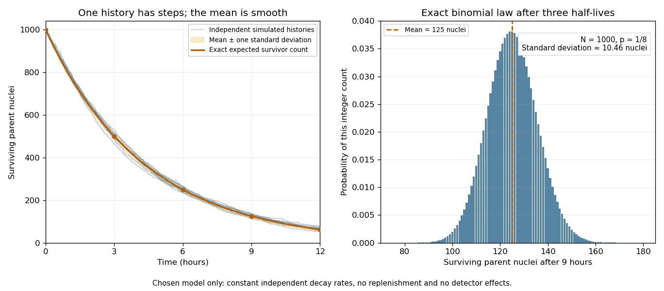
Random survivor counts and the smooth radioactive-decay law
. Original constant-rate model with independent parent atomic nuclei and a half-life. Simulated histories are compared with their exact expected value and a one-standard deviation band. The second panel shows the exact binomial distribution after three half-lives. These are model calculations, not measurements from a historical sample. Details.
In the constant-rate mathematical model, an undecayed atomic nucleus has conditional probabilityof decaying during the next positive interval . The nuclear decay constant has units of inverse time. Its value describes a rate; it does not specify a scheduled death time for one atomic nucleus. The conditional probability is independent of the age , the memorylessness of the exponential distribution.
There are unlisted articles, also show them or only show them.