
The University of California, Santa Barbara's cord demonstration uses a function generator and mechanical driver loosely attached near a clamped cord end. The other end passes over a pulley to a mass hanger, setting tension. Its photograph shows operation with a strobe; the page reports measured and calculated lowest-mode frequencies. Varying drive frequency at fixed loading selects higher normal modes. This clamp arrangement differs from a string tied directly to a moving driver.[ref]
40.75 -- Standing waves on cord (UCSB Department of Physics). Standing waves on cord, opening apparatus description, operating photograph, fixed-end explanation, and calculated versus measured frequency table
A controlled frequency scan holds the cord, endpoint separation and hanging load fixed, then varies frequency slowly to locate large steady amplitudes. Read stationary nodes of a standing wave and count loops; compare the inferred with . As additional checks, compare small drive settings, repeat the scan in reverse, and change only the hanging load to test the predicted square-root tension dependence. These checks test the ideal model rather than adding measurements to the demonstration.
An elastic cord's stretched linear mass density can differ from its relaxed value; the published calculation uses the relaxed value. A strobe can freeze motion at misleading settings, so identify nodes of a standing wave across several snapshots. A moving attachment need not be an exact node of a standing wave. These limits qualify any comparison with ideal fixed-end eigenfrequencies.[ref]
40.75 -- Standing waves on cord (UCSB Department of Physics). Standing waves on cord, clamp and nearby driver distinction, optional strobe, and relaxed-cord linear-density assumption
A stationary mode shape does not imply absence of energy. Write and . For the ideal wave equation on a string, the kinetic energy and elastic potential energy per unit reference length add toHere is signed power crossing a position on the string, positive to the right; is an energy density per length, not per volume. Differentiation and give the local conservation of energy identity . Substitution into givesIt can be nonzero away from a node of a standing wave or an antinode, but its time average over an oscillation period is zero. Energy flows locally back and forth even though this pure standing wave transports no net energy across a section over a complete cycle. At a node of a standing wave, , so kinetic energy density is zero, but need not vanish: elastic potential energy density can be positive there.
For a fixed-end normal mode, integration over givesThe last equality uses . At a straight-string snapshot, while ; at an extreme snapshot, while . This is normal-mode energy exchange. A driven real string with damping requires continuing input power to replace lost energy, so a visually stationary pattern does not establish zero average supplied power.
For the ideal uniform wave equation on a string, the wave speed is , where is constant tension and is linear mass density. Assume small transverse slopes, negligible bending stiffness and no damping. Fix both ends at zero displacement, giving the homogeneous Dirichlet boundary conditions . Our standing wave already satisfies the first. For a nonzero amplitude, the second requires , henceThe value gives zero displacement in this sine family, not a vibrating normal mode. Each positive fits half-wavelengths into the string: it has antinodes, interior nodes of a standing wave, and two endpoint nodes of a standing wave. For and , ; the third normal mode has and wavelength .
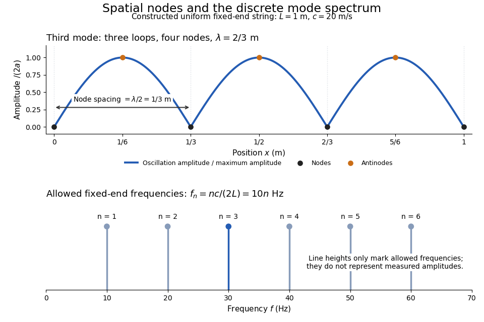
Third-mode nodes and antinodes, with the discrete frequency spectrum of a one-metre ideal string at wave speed twenty metres per second
. Details. 
The equally spaced eigenfrequencies follow from this string's uniform wave speed and fixed-end boundary conditions. They are not a universal spectrum for every vibrating object. Changing an endpoint constraint changes the allowed mode shapes; changing tension changes wave speed. At fixed and , quadrupling doubles every . The more general construction of arbitrary initial motion belongs to normal mode and wave equation on a string.
A node of a standing wave must have for every time, not merely at one snapshot. For , with , set to see that this requires . ThusAn antinode instead maximizes the oscillation amplitude and lies halfway between successive nodes of a standing wave, at . Neighbouring antinodes are also separated by ; the distance from a node of a standing wave to its nearest antinode is . These distances refer to the string's longitudinal coordinate, not its curved arc length.
Within one interval between nodes of a standing wave, all moving points have the same oscillation phase. Adjacent intervals have opposite signs of , so their phase difference is : one loop rises while the next falls. The oscillation phase at an exact node of a standing wave is undefined because its amplitude is zero. A ruler measures the spacing of the fixed pattern; it does not track a moving wave crest.
An excited state can decay by emitting two photons whose energies sum to the transition energy. In hydrogen, this permits the metastable state to reach the ground state during cosmological recombination.
A spin echo refocuses a nucleus's fixed detuning. A nucleus that moves through a magnetic field gradient can have different detunings during the two intervals. To see the distinction without assuming that all noise is reversible, let vary during free evolution. With the same pulse convention, its residual phase at isStatic detuning cancels because . A detuning during the first interval and during the second leaves , which need not vanish. The final component signal is before relaxation; changing the overall receiver convention changes its conjugation but not its magnitude.
For an original quantitative model, take a constant magnetic field gradient and unrestricted one-dimensional Brownian motion , where is the diffusion coefficient and is standard Brownian motion. Then . The constant terms cancel, and the Gaussian distribution of the remaining phase follows from the Brownian covariance kernel . Writing givesThe characteristic function of a zero-mean Gaussian distribution now supplies the extra factor , soHere is in radians per second per tesla, in tesla per metre, and in square metres per second: the extra exponent is dimensionless. The figure chooses , and . With the earlier and , diffusion reduces the echo from to about . These are illustrative model parameters, not values extracted from Hahn's experiment.
This result assumes instantaneous perfect pulses, a constant magnetic field gradient, unrestricted diffusion with constant diffusion coefficient, and independent homogeneous transverse relaxation. Restricted motion, changing gradients, finite pulses and interactions between spins can require different attenuation laws. Even a fixed Hamiltonian is refocused only for the terms whose sign the pulse reverses: a simultaneous 180° rotation of two spins leaves their product unchanged, because both factors change sign. A recovered echo therefore demonstrates a particular recoverable phase history, rather than reversal of every microscopic process.
Erwin Louis Hahn's 1950 apparatus enclosed liquid samples in the coil of a tuned LC circuit, coupled to a gated radio transmitter and radio receiver. One transmitter quadrupled a crystal oscillator's 7.5 MHz to 30 MHz. A separate proton resonance regulator stabilized the static magnetic field.[ref]
Spin Echoes by Erwin Louis Hahn. §IV, Figs. 12–13: transmitter, coil, receiver and regulator
Waiting for thermal equilibrium prepared nuclear polarization. Oscilloscope photographs compared glycerol proton echoes at different field homogeneity: echo width changed; echo time followed twice the pulse separation. Receiver saturation obscured early free induction decay; transmitter leakage required care. The delayed signal tested refocusing; diffusion could still attenuate it.[ref]
Spin Echoes by Erwin Louis Hahn. §II(B), Fig. 2, §IV: preparation, timing, homogeneity comparison and readout limits
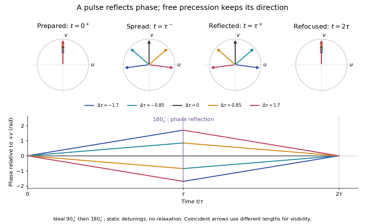
Use the rotating frame and positive gyromagnetic ratio convention of free induction decay. Let be each component's fixed detuning, and normalize its magnetization by the equilibrium value. An instantaneous resonant pulse along rotates through about , preparing . A second pulse along rotates through about . These ideal pulses require a drive much stronger than the relevant detunings and negligible relaxation during either pulse. The corresponding rotation matrices, acting on column vectors, areHere is free Larmor precession in the rotating frame, before including transverse relaxation. Define a calibrated complex signal so the prepared component has . The pulse sends to its negative complex conjugate, hence sends to . Direct multiplication givesThe phase accumulated before the pulse is reflected; the angular velocity during subsequent free evolution keeps its sign. At every fixed detuning has zero residual phase. Equivalently, , so . This is not the identity on arbitrary three-dimensional magnetization: it returns the prepared component because . The two transverse pulse axes specified here also fix the receiver sign of the echo.

For an original ensemble example, let the static detunings have a Gaussian distribution with mean zero and standard deviation , independent of a common homogeneous . Averaging uses the characteristic function of that Gaussian distribution:Choose , and . Immediately before the refocusing pulse the normalized signal is only , yet . A one-pulse free induction decay at 80 ms would instead be about . These chosen numbers describe a calculation, not a measured trace. Increasing narrows the echo without changing in this ideal model. Because this Gaussian distribution produces a Gaussian factor rather than an exponential decay, its inhomogeneous decay is not characterized by a unique exponential .
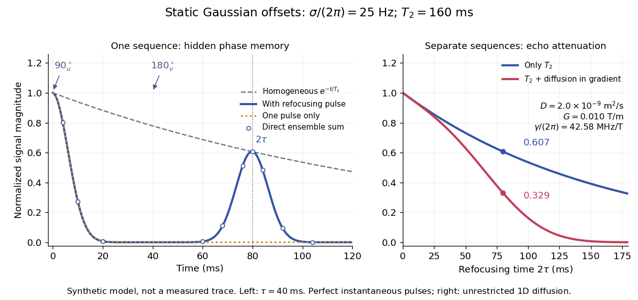

The exact phase-refocusing time is . A slowly falling transverse relaxation envelope moves the maximum of this particular echo shape slightly earlier: differentiating after the pulse gives , or here. Measuring consistently at avoids confusing this small envelope effect with a failure of refocusing. A series of such measurements gives only when the assumed homogeneous exponential decay, pulse quality and negligible additional attenuation are appropriate.
For a spherical shell of uniform mass density , inner radius and outer radius , suppose a negligible-width radial tunnel permits a small mass to fall from rest at the outer surface. The enclosed mass at radius within the material is . The spherical shell theorem gives inward gravitational acceleration . Integrating from to gives released gravitational potential energy , hence speed at the cavity. The cavity has zero gravitational field, so the diameter transit time is the title expression, independent of and .
The Sagnac effect is a difference in return times, or an associated interference fringe displacement, for light sent in opposite directions around a closed optical path in a rotating apparatus. The light leaves one beam splitter, travels around the same loop in opposite senses, and returns to the rotating beam splitter and readout. For a slowly rotating apparatus in flat spacetime, the leading laboratory arrival-time difference isHere is the vacuum speed of light, is the apparatus's angular velocity relative to an inertial frame, and is the vector area oriented by the chosen positive direction around the closed curve . With positive rotation about the upward normal vector, the counterclockwise beam is labelled and arrives later. Reversing rotation, or reversing the orientation convention alone, changes the sign of .
The surprise is that a small loop can reveal its rotation by comparing two beams locally, even though each local vacuum speed of light measurement gives . A rotating reference frame is not a single inertial frame: a beam must catch the moving receiver after a full circuit. The Sagnac area law makes this difference a practical way to measure angular velocity, while the Relativistic Sagnac delay on a circular ring distinguishes laboratory coordinate time from the receiver's proper time.
For a particle instantaneously at rest in a primed frame moving at relative to the laboratory, the ordinary three-force transforms as and . The spatial components of the four-force are , whereas its time component is . For a co-moving material segment, length contraction also changes its laboratory length, so transforming total force is not the same as transforming force per unit length.
Thomas precession is the kinematic rotation arising when the successive instantaneous rest frames of an accelerated particle are connected by noncollinear Lorentz boosts. Its contribution is needed in deriving the leading atomic spin-orbit coupling: for an electron in central potential energy , the corrected term is . A rest-field argument alone gives twice this coefficient.[ref]
Topics in Quantum Mechanics by David Tong. §3.1.3, printed pp. 71–75, especially the correction from the accelerated electron frame
Special relativity connects measurable clock rates, length contraction, light propagation, and four-momentum through the Lorentz transformation. Tests probe particular predictions rather than measuring a coordinate transformation in isolation. Examples include cosmic-ray muon time-dilation experiments, muon storage-ring time-dilation experiments, the Michelson-Morley experiment, the Fizeau experiment, and particle-collision energy and momentum balances.
The first postulate is Einstein's principle of relativity: nongravitational laws have the same form in every inertial frame. The second states that light in vacuum propagates at the same finite speed of light in every inertial frame, independently of the source's motion. Together with the usual spacetime symmetries and calibrated coordinates, these postulates yield the Lorentz transformation. The relativity principle alone also admits the Galilean transformation with its infinite invariant-speed limit.
Filtration separates suspended solid particles from a fluid using a porous barrier. Dissolved ions can pass with the fluid; the separation does not establish the filtrate's composition. Solubility product measurement by titration requires removal of undissolved calcium hydroxide before acid-base titration.
An ideal solution is a chemical solution whose component chemical potentials depend on composition throughHere is an amount of substance, its mole fraction, the molar gas constant, and the pure-component liquid reference at the same temperature and pressure . This model applies to every component across the composition range; it is stronger than an approximation valid only near a pure solvent.[ref]
With this pure-liquid standard state convention, the thermodynamic activity satisfies , so an ideal solution has , or activity coefficient .[ref]
ideal mixture. IUPAC Compendium of Chemical Terminology, fifth edition (Gold Book) by International Union of Pure and Applied Chemistry; Ideal mixture, definition: activities equal mole fractions, equivalently unit activity coefficients; I02938, online version 5.0.0
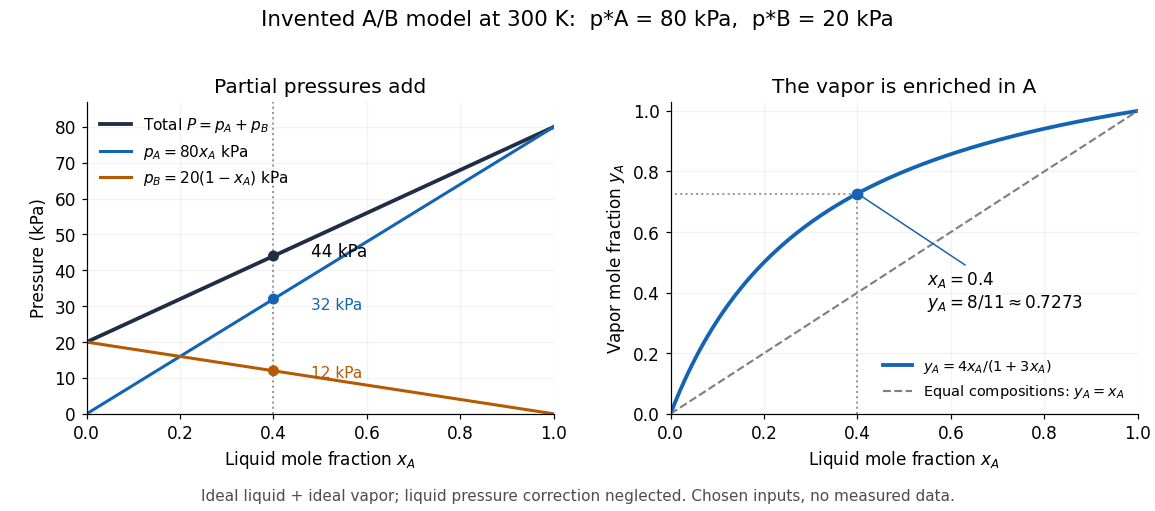
This statement concerns the liquid. Assuming that a coexisting vapor is an ideal gas mixture is an additional approximation. Its mole fractions generally differ from the liquid mole fractions .For an original two-component example, stipulate and pure-component vapor pressures and . A and B are invented distinguishable components; these numbers are chosen model inputs, not material data. Combine an ideal solution with an ideal gas vapor, neglect the pure-liquid reference's pressure correction, and exclude other gases. At liquid mole fractions and , Raoult's law and addition of partial pressures giveThus the coexisting vapor contains about A by amount of substance, although the liquid contains only . The total pressure is neither pure-component vapor pressure, and cannot be substituted for . This enrichment is the basis of distillation.

The usefulness of the ideal solution is that one composition law connects chemical potentials, vapor-liquid equilibrium, entropy of mixing and Gibbs free energy of mixing. Its liquid components can interact strongly: the defining condition is their composition dependence, rather than the absence of all interactions as in an ideal gas model.
A chemical solution with a polymer as a solute. The polymer conformation and interactions depend on the solvent and concentration.
Test coverage measures which selected program elements a test run exercises. Statement coverage counts executed statements; branch coverage counts executed control-flow alternatives. Exercising both sides of a conditional can reveal gaps missed by statement coverage, but even full branch coverage need not exercise all paths or meaningful value combinations. Coverage records execution, not whether assertions checked the right behaviour. A suite that calls every function and verifies nothing can have impressive coverage while failing to detect wrong results.
There are unlisted articles, also show them or only show them.