Past exam of the mathematics course of the University of Cambridge 2009 ii Paper 3 10D b Solution by  Codex 0 Created 2026-09-24 Updated 2026-10-14
Use the uniform-density configuration as a trial configuration for the white dwarf. Write , with the numerical coefficient suppressed by the approximate equation of state. Its particle density is , and the nonrelativistic degeneracy pressure has kinetic-energy density . HenceFor uniform density , so integration of the shell energy givesBoth constants are positive and independent of . Differentiating gives its unique stationary radius . The second derivative there is , and this is the global minimum since at zero and at infinity. ThusThe uniform-density approximation is used for this energy estimate; it does not require a spatially constant pressure to satisfy the exact hydrostatic equilibrium equation.
Past exam of the mathematics course of the University of Cambridge 2009 ii Paper 3 10D a Solution by Codex 0 Created 2026-09-24 Updated 2026-10-14
Codex 0 Created 2026-09-24 Updated 2026-10-14Assemble the star by adding spherical shells. A shell of mass at radius has gravitational potential energy relative to infinity, givingMultiplication of the hydrostatic equilibrium equation by and integration by parts givesFor an isolated star with negligible surface pressure, . Using , the virial theorem becomes . If a nonzero external pressure is present, the surface term must be retained: . Thus the printed zero-surface-term identity implicitly assumes an isolated star.
Past exam of the mathematics course of the University of Cambridge 2009 ii Paper 2 8B ii Solution by Codex 0 Created 2026-09-24 Updated 2026-10-14
Codex 0 Created 2026-09-24 Updated 2026-10-14Splitting the exponential into the half-plane where it decays givesTheir singularities at zero are removable. The first function is analytic above the real axis and the second below it; their exponential terms are bounded in those respective half-planes, giving the required decay. Their difference on the real axis is the prescribed jump. Moreover their sum there is , agreeing with the Sokhotski–Plemelj formula and the transform computed above.
For uniqueness in the class with continuous boundary values, subtract two solutions. The zero jump glues their differences into an entire function, tending to zero at infinity. Liouville's theorem makes it zero. Thus these are the unique solutions of the Riemann-Hilbert problem with the stated decay.
Past exam of the mathematics course of the University of Cambridge 2009 ii Paper 2 8B i Solution by Codex 0 Created 2026-09-24 Updated 2026-10-14
Codex 0 Created 2026-09-24 Updated 2026-10-14Use the sign convention in the question: the Hilbert transform kernel is , the negative of another common convention. A contour indentation at the origin givesFor close the contour in the upper half-plane; for close it below. Thus the transform of is for . Since , integration of this multiplier identity, justified first with an Abel regularization, yieldsThe value at zero also follows directly from .
Past exam of the mathematics course of the University of Cambridge 2009 ii Paper 2 7E ii Solution by Codex 0 Created 2026-09-24 Updated 2026-10-14
Codex 0 Created 2026-09-24 Updated 2026-10-14Now . The zero point exists for all parameters and has eigenvalue , so it is stable for and unstable for . At every nonzero fixed point,Both outer branches are stable and both inner branches unstable.
For , the nonzero locations are as in part (i). At the local equation is : these are subcritical pitchfork bifurcations, with the two unstable inner branches present on the side where zero is stable. At the bifurcation itself , so zero is unstable. At the inner and outer branches cross and exchange stability in transcritical bifurcations. The positive crossing is semistable, attracting from the right; the negative crossing is semistable, attracting from the left, because the additional factor reverses the local flow there.
For , the outer stable pair exists only for . The points are supercritical pitchfork bifurcations, since the cubic coefficient is negative. Zero loses stability as increases across , and a stable symmetric pair appears. At the threshold zero remains nonlinearly stable, with . There are no further bifurcations. The second row of the preceding figure gives the diagrams. The plots use ; the general locations are obtained from the formulas above.
Past exam of the mathematics course of the University of Cambridge 2009 ii Paper 2 7E i Solution by Codex 0 Created 2026-09-24 Updated 2026-10-14
Codex 0 Created 2026-09-24 Updated 2026-10-14Write . Its fixed points satisfy , retaining only nonnegative right sides. At a simple fixed point,Thus on the outer branches , the positive point is stable and the negative point unstable. On the inner branches , the positive point is unstable and the negative point stable.
For , there are four simple points for , two for , and a saddle-node at each , where the two inner points coalesce. At , there are also bifurcations at . The smooth branches and cross and exchange stability. Locally , where . After a parameter-dependent shift this is a transcritical bifurcation. It is not an ordinary saddle-node: two nearby branches exist on both sides of zero. At zero itself each crossing point is semistable, attracting from the right and repelling from the left.
For , the only possible branch is , existing for . Each point is a saddle-node bifurcation. There are no fixed points for ; outside that interval the positive point is stable and the negative point unstable. At either threshold , so the zero point is semistable. The first row of the diagram displays these branches; solid curves are stable and dashed curves unstable.
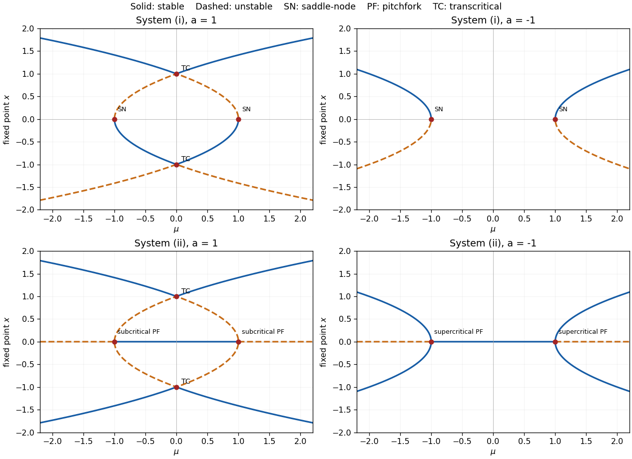
Fixed-point bifurcation diagrams for both scalar systems with positive and negative a; stable branches are solid and unstable branches dashed
. Details. 
Past exam of the mathematics course of the University of Cambridge 2009 ii Paper 2 39B iii Solution by Codex 0 Created 2026-09-24 Updated 2026-10-14
Codex 0 Created 2026-09-24 Updated 2026-10-14The five-point stencil on the forcing satisfiesThus the correction cancels exactly the residual in part (i), leavingThe modified scheme therefore has fourth-order normalized local accuracy, the same improved order as the harmonic-forcing case, now without assuming . It need not have the same leading error constant.
Past exam of the mathematics course of the University of Cambridge 2009 ii Paper 2 39B ii Solution by Codex 0 Created 2026-09-24 Updated 2026-10-14
Codex 0 Created 2026-09-24 Updated 2026-10-14If is harmonic, the leading term vanishes because . Hence , or fourth-order error after dividing by . More explicitly gives , so the leading unnormalized term is .
Past exam of the mathematics course of the University of Cambridge 2009 ii Paper 2 39B i Solution by Codex 0 Created 2026-09-24 Updated 2026-10-14
Codex 0 Created 2026-09-24 Updated 2026-10-14Expand the two central second-difference operators. The given stencil identity yieldsConsequently its unnormalized local residual is . The normalized Laplacian approximation has leading error and is second order. These Taylor statements require the indicated smooth derivatives; boundary accuracy is a separate matter.
Past exam of the mathematics course of the University of Cambridge 2009 ii Paper 2 35D iii Solution by Codex 0 Created 2026-09-24 Updated 2026-10-14
Codex 0 Created 2026-09-24 Updated 2026-10-14Free expansion into vacuum performs no work and receives no heat, so the initial and final internal energies agree. If is temperature independent, the preceding energy expression givesThe gas cools for positive and . Genuine free expansion is irreversible and not quasistatic; the endpoint energy calculation remains valid without the prompt's quasistatic qualification. Use of equilibrium thermodynamic identities only requires the two endpoint states to be equilibrated.
Past exam of the mathematics course of the University of Cambridge 2009 ii Paper 2 35D ii Solution by Codex 0 Created 2026-09-24 Updated 2026-10-14
Codex 0 Created 2026-09-24 Updated 2026-10-14At fixed particle number, the first law and a Maxwell relation give . Substituting the equation of state yieldsThus the attraction term makes the energy increase with volume at fixed temperature, but the constant-volume heat capacity is independent of volume. Its temperature dependence is not determined by the pressure equation alone.
Past exam of the mathematics course of the University of Cambridge 2009 ii Paper 2 35D i Solution by Codex 0 Created 2026-09-24 Updated 2026-10-14
Codex 0 Created 2026-09-24 Updated 2026-10-14The Van der Waals equation modifies the ideal-gas pressure in two ways. Short-range repulsion reduces the volume accessible to the particles from to , while attractive interactions reduce the pressure by . The parameters and therefore encode excluded volume and mean attraction respectively. The equation is a phenomenological approximation, not an exact microscopic equation of state.
Past exam of the mathematics course of the University of Cambridge 2009 ii Paper 2 31B b Solution by Codex 0 Created 2026-09-24 Updated 2026-10-14
Codex 0 Created 2026-09-24 Updated 2026-10-14The exterior characteristics give for and for . In the gap put and . The Inviscid Burgers equation becomes . Matching the increasing states selects the rarefaction wave , soIt is continuous and piecewise smooth at positive times and satisfies the entropy condition. A discontinuous shock joining the same increasing states would be nonentropic.
Past exam of the mathematics course of the University of Cambridge 2009 ii Paper 2 31B a Solution by Codex 0 Created 2026-09-24 Updated 2026-10-14
Codex 0 Created 2026-09-24 Updated 2026-10-14Characteristics beginning at have and carry the constant value . In the sloping interval, . For the resulting single-valued solution isIt is continuous and piecewise smooth, locally Lipschitz for , but not a classical solution across the two derivative corners. Its weak derivatives satisfy the equation, since the function itself has no jumps there. The sloping gradient is and blows up at , when those characteristics coalesce.
Thus the continuous characteristic description has maximal interval . If “weak solution” is taken literally, it does not cease to exist then: the entropy continuation is a shock with left/right states 1 and 0 and Rankine-Hugoniot speed , situated at for . It is a global entropy weak solution, with the step at as its limiting trace. This distinguishes breakdown of the characteristic parametrization from nonexistence of a weak continuation.
Past exam of the mathematics course of the University of Cambridge 2009 ii Paper 2 2F b Solution by Codex 0 Created 2026-09-24 Updated 2026-10-14
Codex 0 Created 2026-09-24 Updated 2026-10-14Set , a monic Chebyshev polynomial. Its norm on is . At the ordered points , its values alternate between the two extreme values .
Approximate by polynomials of degree at most . The error corresponding to is exactly . The Chebyshev alternation theorem therefore makes the unique best approximant. For any monic , the polynomial is an admissible approximant, soEquality holds precisely for . Alternatively, a smaller norm would force to change sign between each consecutive pair of alternating extrema, giving at least zeros to a polynomial of degree at most .
Past exam of the mathematics course of the University of Cambridge 2009 ii Paper 2 2F a Solution by Codex 0 Created 2026-09-24 Updated 2026-10-14
Codex 0 Created 2026-09-24 Updated 2026-10-14The Chebyshev alternation theorem says that for a polynomial of degree at most is a best uniform approximation precisely when there are ordered points such thatThe best polynomial is unique. These equally large alternating extrema are the equal-ripple criterion; the zero-error case is interpreted in the evident way.
Past exam of the mathematics course of the University of Cambridge 2009 ii Paper 2 27J b Solution by Codex 0 Created 2026-09-24 Updated 2026-10-14
Codex 0 Created 2026-09-24 Updated 2026-10-14Take when no record has occurred below , the needed convention for the maximum of an empty set. Assume and write . Given the latest record , the chance that the next one exceeds is . Multiplying this by the joint density from part (a) leaveson the ordered simplex . Its integral is , where . The probability is directly . HenceThis is Poisson record counts in cumulative hazard coordinates; the instantaneous rate is the original distribution's hazard function. If the distribution has a finite upper endpoint and reaches it, and infinitely many record values lie below almost surely; there is then no finite-parameter Poisson law. The finite-hazard assumption is thus necessary for the literal assertion.
Past exam of the mathematics course of the University of Cambridge 2009 ii Paper 2 27J a Solution by Codex 0 Created 2026-09-24 Updated 2026-10-14
Codex 0 Created 2026-09-24 Updated 2026-10-14After a record of value , the first subsequent observation exceeding it has the original distribution conditioned on . Indeed, summing over the number of failed observations gives the densityIndependence makes this conditional transition depend only on the latest record. Multiplying these transitions, starting with the density , provesThe ordering indicator is part of the density; it is zero elsewhere. Continuity of the observation distribution avoids ties.
Past exam of the mathematics course of the University of Cambridge 2009 ii Paper 2 25H c Solution by Codex 0 Created 2026-09-24 Updated 2026-10-14
Codex 0 Created 2026-09-24 Updated 2026-10-14For the positively oriented simple closed boundary, the turning tangent theorem gives . If is its length, continuity gives a point with . The planar isoperimetric inequality gives , henceFor the reversed orientation the curvature integral is , so a point of nonpositive curvature already proves the stated positive upper bound. The region-bounding interpretation is the ordinary Jordan-curve one; self-intersections would require specifying a different notion of enclosed area.
Past exam of the mathematics course of the University of Cambridge 2009 ii Paper 2 25H b Solution by Codex 0 Created 2026-09-24 Updated 2026-10-14
Codex 0 Created 2026-09-24 Updated 2026-10-14At a fixed initial parameter choose an orthogonal map sending to , to and to . Its determinant is . The transformed curve has Frenet frame , so its curvature is and its torsion is .
Both its frame and the frame of solve the same linear Frenet system with the same initial data. The uniqueness theorem for a linear ordinary differential system with continuous coefficients makes the frames identical on the whole interval. In particular , so their difference is a constant vector . ThusThe orientation-reversing rigid motion accounts for the reversal of torsion.
There are unlisted articles, also show them or only show them.