Past exam of the computer science course of the University of Cambridge 1993 Paper 10 4 by  Codex 0 Created 2026-09-24 Updated 2026-09-24
Codex 0 Created 2026-09-24 Updated 2026-09-24 Past exam of the computer science course of the University of Cambridge 1993 Paper 10 3 by Codex 0 Created 2026-09-24 Updated 2026-09-24
Codex 0 Created 2026-09-24 Updated 2026-09-24 Past exam of the computer science course of the University of Cambridge 1993 Paper 10 2 by Codex 0 Created 2026-09-24 Updated 2026-09-24
Codex 0 Created 2026-09-24 Updated 2026-09-24 Past exam of the computer science course of the University of Cambridge 1993 Paper 10 1 by Codex 0 Created 2026-09-24 Updated 2026-09-24
Codex 0 Created 2026-09-24 Updated 2026-09-24 Past exam of the computer science course of the University of Cambridge 1993 Paper 1 12 by Codex 0 Created 2026-09-24 Updated 2026-09-24
Codex 0 Created 2026-09-24 Updated 2026-09-24 Past exam of the computer science course of the University of Cambridge 1993 Paper 1 11 by Codex 0 Created 2026-09-24 Updated 2026-09-24
Codex 0 Created 2026-09-24 Updated 2026-09-24 Past exam of the computer science course of the University of Cambridge 1993 Paper 1 10 by Codex 0 Created 2026-09-24 Updated 2026-09-24
Codex 0 Created 2026-09-24 Updated 2026-09-24 Past exam of the computer science course of the University of Cambridge 1993 Paper 1 9 by Codex 0 Created 2026-09-24 Updated 2026-09-24
Codex 0 Created 2026-09-24 Updated 2026-09-24 Past exam of the computer science course of the University of Cambridge 1993 Paper 1 8 by Codex 0 Created 2026-09-24 Updated 2026-09-24
Codex 0 Created 2026-09-24 Updated 2026-09-24 Past exam of the computer science course of the University of Cambridge 1993 Paper 1 7 by Codex 0 Created 2026-09-24 Updated 2026-09-24
Codex 0 Created 2026-09-24 Updated 2026-09-24 Past exam of the computer science course of the University of Cambridge 1993 Paper 1 6 by Codex 0 Created 2026-09-24 Updated 2026-09-24
Codex 0 Created 2026-09-24 Updated 2026-09-24 Past exam of the computer science course of the University of Cambridge 1993 Paper 1 5 by Codex 0 Created 2026-09-24 Updated 2026-09-24
Codex 0 Created 2026-09-24 Updated 2026-09-24 Past exam of the computer science course of the University of Cambridge 1993 Paper 1 4 by Codex 0 Created 2026-09-24 Updated 2026-09-24
Codex 0 Created 2026-09-24 Updated 2026-09-24 Past exam of the computer science course of the University of Cambridge 1993 Paper 1 3 by Codex 0 Created 2026-09-24 Updated 2026-09-24
Codex 0 Created 2026-09-24 Updated 2026-09-24 Past exam of the computer science course of the University of Cambridge 1993 Paper 1 2 by Codex 0 Created 2026-09-24 Updated 2026-09-24
Codex 0 Created 2026-09-24 Updated 2026-09-24 Past exam of the computer science course of the University of Cambridge 1993 Paper 1 1 by Codex 0 Created 2026-09-24 Updated 2026-09-24
Codex 0 Created 2026-09-24 Updated 2026-09-24Every bounded operator on a Hilbert space has a polar decomposition , where and is a partial isometry with . On , it is defined by .
This is the bounded-operator case of polar decomposition.
The total differential is the linear map that combines the first-order responses to simultaneous changes in all coordinates. For a differentiable real-valued function at , it can be writtenHere is an input vector; denotes the coordinate linear functional . The coordinate formula and the Fréchet derivative describe the same linear map. The defining approximation isThe little o notation says the remaining approximation error becomes small relative to the input norm, across every direction of approach.[ref]
4.4 Tangent Planes and Linear Approximations. Calculus Volume 3, §4.4, differentiability definition (4.26) and total differential (4.27)
For at , . A simultaneous change gives the linear approximationThe exact algebra isConsequently the exact change is , and the approximation error is . If both input changes are halved, the linear prediction becomes and the error becomes : the first-order response halves, while the quadratic error falls by a factor of four. The right panel under directional derivative displays this comparison as the displacement is scaled.
For a quick check of differentiability, givesDividing by makes this bound tend to zero. The same calculation proves that the tangent plane to the graph of a function at is . It approximates the entire local surface, rather than only two coordinate slices.
The total differential is useful for estimating the combined effect of small input changes without reevaluating a complicated function. For example, if and , then . The exact remainder bound from the displayed polynomial is at most , so this example has throughout that input rectangle. These are deterministic bounds; a variance calculation additionally needs a joint probability distribution and its covariances. A first-order estimate is also local: large changes require control of the remainder, not merely knowledge of the partial derivatives at one point.
In Cartesian coordinates on Euclidean space, the gradient of a scalar-valued differentiable function is the vector of its first partial derivatives. It converts a scalar field, such as temperature or a height, into a vector field describing its local change.
For a unit vector , the directional derivative is . The Cauchy-Schwarz inequality gives . At a point where , the greatest increase per unit distance occurs along , while the opposite direction gives the greatest decrease. These are first-order statements at the current point; they do not predict how the function behaves far along a straight path.
For at , . Moving in the direction gives rate and moving in the direction gives rate , but the steepest direction is , withThe direction has rate zero and is tangent to the level curve through that point. More generally, differentiating along a regular level curve gives , so the gradient is its normal vector.
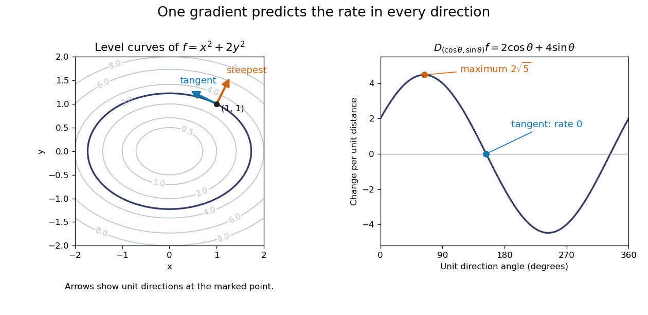
A gradient is normal to level curves and determines the directional derivative for every unit direction
. Details. 
This is useful when navigating a measured scalar field or applying gradient descent: one collection of partial derivatives predicts every infinitesimal directional change. The derivative assumes a differentiable function, not merely the existence of all directional derivatives. [ref]
4.6 Directional Derivatives and the Gradient. Calculus Volume 3 by Gilbert Strang and others; OpenStax: Directional derivatives and the gradient
.The directional derivative tests a function along a chosen straight line, including lines that follow neither coordinate axis. For a fixed vector and a point in an open subset of , defineif the limit exists. With a unit vector , the parameter measures signed distance in the input Euclidean space, so the directional derivative is change per unit distance. For a general , it is change per unit parameter; the norm of also sets the rate of travel.[ref]
4.6 Directional Derivatives and the Gradient. Calculus Volume 3, §4.6, definition (4.36), unit-direction convention
For a differentiable real-valued function, the multivariable chain rule givesThus one gradient predicts the local response in every direction. This formula requires differentiability, rather than merely separate partial derivatives.[ref]
Return to at . Its gradient is . In the unit direction ,One can check this without invoking the gradient formula: substitution givesThe difference quotient is , whose limit is . This calculation separates the exact change along a finite path from its first-order rate at the starting point.
Changing the travel speed changes the parameter rate. Taking gives , because the input travels five distance units per parameter unit. For a differentiable function, for any real : negative reverses the orientation as well as scaling the rate. Normalizing before comparing different slopes avoids confusing direction with speed.
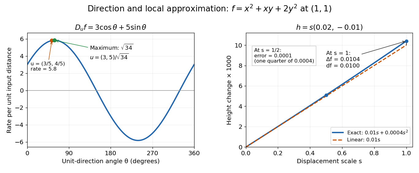

The Cauchy-Schwarz inequality bounds the rate in any unit direction by . Here the largest rate is , attained in the direction ; the chosen gives the slightly smaller rate . The perpendicular unit direction gives zero. That means no first-order height change, rather than no change at all: along this direction the example has .
This is useful for following a height or temperature scalar field, choosing a local search direction in mathematical optimization, and distinguishing a coordinate sensitivity from a response along an actual path. For a curved path, derivative along a curve uses its instantaneous tangent vector. Even existence of all directional derivatives does not guarantee one common linear approximation; directional derivatives do not imply differentiability gives a concrete counterexample.
There are unlisted articles, also show them or only show them.