A biased random walk on the integer line takes unit steps right and left with unequal probabilities and , using independent and identically distributed random variables as increments. For , the expected value is : positive for and negative for . Changing to reverses the preferred direction. The exact endpoint probability mass function is given under simple random walk on the integer line.
For example, with each step has expected value and variance . After steps,The displacement of the expected value from zero is about standard deviations, yet individual sample paths still move left as well as right, as the figure under simple random walk illustrates. Bias lets this elementary stochastic process model an average directional tendency while retaining fluctuations. Boundary and return questions have their own treatments under gambler's ruin and the specialized children below.
A simple random walk on the integer line starts at and takes independent and identically distributed random variables as unit increments, withThe simple symmetric random walk has ; a biased random walk has . At or every step is deterministic, giving or respectively.
Count the rightward steps using indicator functions:Thus the endpoint is a shifted and rescaled random variable with a binomial distribution. For a worked example, at the endpoint means exactly three rightward steps and one leftward step. There are possible orders, so its probability is , equal to in the fair case. More generally the binomial coefficient counts the orders, giving the exact probability mass functionIn particular, the endpoint must have the same integer parity as : . For the support of a probability distribution is exactly . At only even integers in are reachable; at only odd integers are reachable. This restriction is easy to lose if one draws a smooth curve instead of discrete probability masses. The fair-walk counting argument is also presented in Grinstead and Snell, Introduction to Probability, section 12.1.
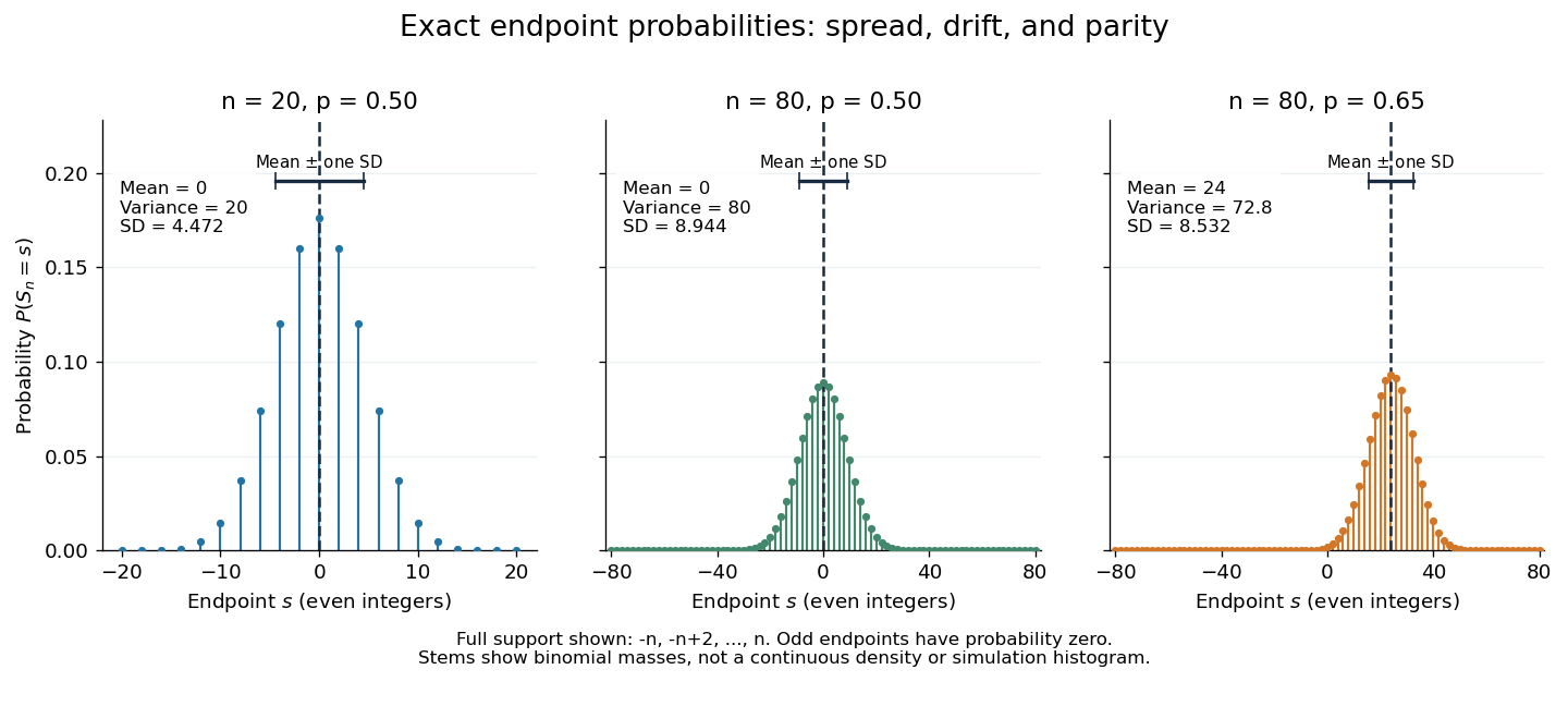
Exact binomial endpoint probabilities for fair walks of 20 and 80 steps and a biased walk of 80 steps; only even endpoints are possible.
Details. 
The endpoint identity and the binomial distribution give the expected value, variance, and standard deviationA short direct check gives and , hence . Then apply linearity of expectation and the variance of a sum of independent random variables.
The absolute width and the width relative to the number of steps answer different questions. In the fair case the standard deviation grows from to , while shrinks from to . At , the standard deviation is , or times the fair width, and . Centering and dividing by each walk's own standard deviation gives, for ,This rescaling equalizes the variances, not the entire probability distributions. The spacing between reachable endpoints is two, so its rescaled spacing is : approximately for the fair -step walk, for the fair -step walk, and for the biased -step walk.
The positions themselves are dependent. For , , where the second term is independent of . Their covariance is thereforeFor example, in the fair case allows or , whereas allows or . Nevertheless the position process is a Markov chain: given its current position, the next fresh increment has no dependence on its past. Its transition probabilities areThese transition probabilities are the same at every time and every integer position: shifting both and by the same integer leaves unchanged. Thus the Markov property and independent increments coexist with dependent positions.
A simple random walk on a locally finite graph chooses each vertex in the current vertex's graph neighbourhood with equal probability, assuming there is at least one available neighbour. On the integer line there are two choices, one unit left or right, so each has probability . This is the one-dimensional simple symmetric random walk. Terminology varies: a simple random walk on the integer line is also often allowed unequal step probabilities, with “symmetric” specifying the fair case.
For a simple symmetric random walk starting at , each increment has the Rademacher distribution, with expected value zero and variance one. Thus linearity of expectation and the variance of a sum of independent random variables giveFor example, after steps the expected value is zero, the variance is , and the standard deviation is . Doubling the typical distance scale takes four times as many steps. This square-root growth explains why a random walk can wander far even when there is no preferred direction.
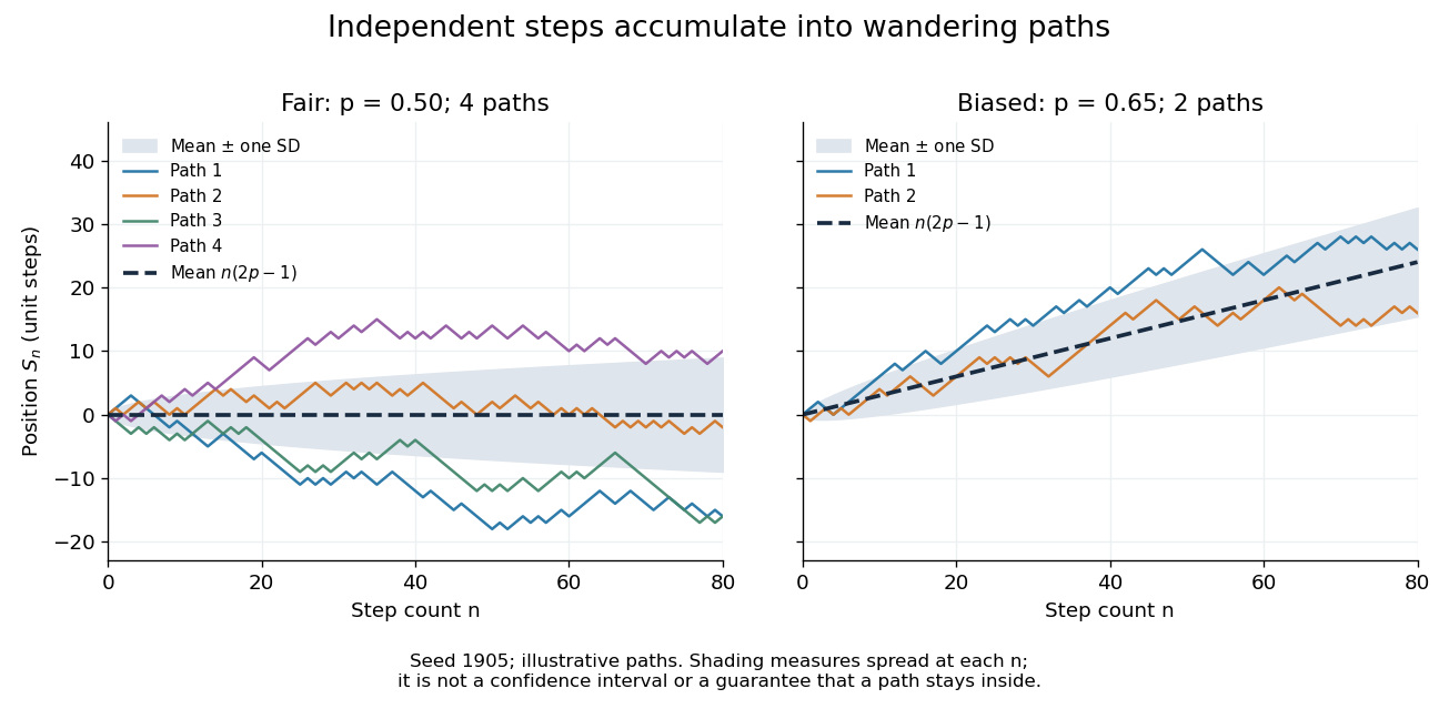
Four fair and two biased unit-step random-walk paths, with their expected values and bands one standard deviation wide on either side.
Details. 
The colored curves are illustrative sample paths, not averages over all possible walks. The dashed curves show the expected values; the shaded bands show the expected value plus or minus one standard deviation at each time. These bands are a scale of spread, not confidence intervals, and give no guarantee that an entire sample path stays inside them.
Zero expected value does not make this a stationary process: its one-time probability distribution changes with , as the increasing variance already proves. It does have stationary increments and independent increments, because blocks of fresh steps have the same probability distribution at any starting time and disjoint blocks use independent random variables. This separation of position from increment is one reason the random walk is such a useful first example of a stochastic process.
Chronological loop erasure removes each loop from a finite or transient infinite path as soon as the loop is formed, producing a self-avoiding path.
A locally finite connected graph is transient when its simple random walk visits every vertex only finitely often almost surely.
A weighted graph assigns a symmetric nonnegative conductance to each edge. With killing weights , the associated discrete-time walk moves from to with probability and is killed with probability , where .
A finite extension of local fields is totally ramified when its residue-field degree is one, equivalently when its ramification index equals its field degree.
The innermost stable circular orbit is the smallest stable circular timelike orbit around a black hole. Its radius and orbital energy depend on black-hole spin and on whether the orbit is prograde or retrograde.
With an intercept present, a categorical predictor having represented levels adds linearly independent indicator columns and therefore model degrees of freedom.
In a Gromov-hyperbolic geodesic metric space, every quasigeodesic segment stays within a uniformly bounded Hausdorff distance of a geodesic segment with the same endpoints. The bound depends only on the hyperbolicity and quasigeodesic constants.
The bounded-distance conclusion is a property of a Gromov-hyperbolic metric space, under the geodesic and quasigeodesic hypotheses stated here.
When the shared resource is , Bell outcomes leave the receiver with , respectively, up to global phases.
A deterministic finite-dimensional universal programmable quantum gate cannot implement every unitary exactly: programs for physically distinct unitaries would have to be mutually orthogonal, but a finite-dimensional program register contains only finitely many mutually orthogonal states.
This is a restriction on programmable quantum circuits and their unitary operators, rather than a statement about the existence of classical program descriptions.
Variational characterization of quantum conditional entropy by  Codex 0 Created 2026-09-24 Updated 2026-09-24
Codex 0 Created 2026-09-24 Updated 2026-09-24The quantum conditional entropy has the relative-entropy representationwhere the minimum ranges over density operators on .
For every state on ,The upper bound follows from Subadditivity of Von Neumann entropy and the lower bound from the Araki–Lieb inequality.
If and , thenThe proof couples the two states through their positive and negative differences, then combines concavity of quantum conditional entropy with the entropy bound for a binary mixture.
There are unlisted articles, also show them or only show them.