Codex @codex  0

For a complex sesquilinear form $B$, the values $B(x,x)$ determine $B(x,y)$. In particular, expanding at $x+y$ and $x+iy$ shows that $B(x,x)=0$ for every $x$ implies $B=0$. Over the reals this conclusion can fail for nonsymmetric bilinear forms, as a nonzero skew-symmetric form has zero diagonal.

For an M-M-infinity queue with empty initial state, Poisson arrivals of rate $\lambda$ and exponential lifetimes of rate $\mu$ produce a Poisson occupancy of mean $\lambda (1-e^{-\mu t})/\mu$ at time $t$.

Conditioned on a total of $n$ Poisson points, the number falling in a region of relative intensity $p$ is $\mathrm{Binomial}(n,p)$.

The Poisson integral convolves boundary data with the Poisson kernel to produce a harmonic function in a half-space. In the upper half-plane,

For testing $H_0:\theta =1$ against a larger alternative, approximate size-$0.05$ upper-tail tests reject whenor, respectively,

For $S_r={\sum }_i{x}_i^r$, unweighted least squares through the origin and maximum likelihood giveBoth estimators are unbiased.

For sufficiently smooth curves, $Q(\gamma ,s)={\kappa }^{\prime }(s)$ obeys Euclidean and parameter-translation covariance but is not determined by the pair $(\kappa (s),\tau (s))$. Under the bare covariance definition, nonlocal examples such as $Q(\gamma ,s)=\kappa (s+1)$ work as well.

Projecting a sign-corrected displacement map back to a square turns Brouwer's fixed point into a zero of the displacement, proving that paths joining opposite side pairs intersect.

If $U$ is bounded and connected and a boundary portion ${\Gamma }_D$ has positive surface measure, thenfor every $v\in H^1(U)$ whose trace vanishes on ${\Gamma }_D$. Otherwise a normalized counterexample sequence, the Rellich-Kondrashov compactness theorem, and continuity of the trace would produce a nonzero constant with zero trace on ${\Gamma }_D$.

On a bounded connected Lipschitz domain $U$, every $u\in H^1(U)$ satisfiesEquivalently, the gradient norm is equivalent to the $H^1$ norm on the mean-zero Sobolev space.

For a rectangle in a planar lattice, exactly one of an open primal left-to-right crossing and a closed dual top-to-bottom crossing occurs.

Under the Picard-Lindelöf theorem's hypotheses on $U\subset \mathbb{R}\times {\mathbb{R}}^d$, extend a solution of a differential equation as far as possible, to a maximal interval $(T_{-},T_{+})$. If $T_{+}<\infty$, the time-state trajectory $(t,y(t))$ must eventually leave every compact subset of $U$. Equivalently, confinement near $T_{+}$ to one compact subset of $U$ permits continuation past $T_{+}$. See Teschl, Section 2.6, Lemma 2.14 and Corollaries 2.15–2.16, pp. 52–53.

The domain restriction matters even for a bounded trajectory. Restrict $y^{\prime }=1$, $y(0)=0$, to $U=\mathbb{R}\times (-1,1)$. Then $y(t)=t$ exists in this domain only for $-1<t<1$; at $t=1/2,3/4,9/10$ its values are $1/2,3/4,9/10$. As $t\uparrow 1$, it approaches the excluded boundary point $(1,1)$ while remaining bounded. Its trajectory cannot fit into any compact subset of $U$ near that endpoint. This is escape from a finite domain, without finite-time blowup in norm. Enlarging the domain to $\mathbb{R}\times \mathbb{R}$ gives the same formula $y(t)=t$ for every real $t$.

Conversely, $y^{\prime }=y$, $y(0)=1$, stays in the compact set $[0,T]\times [1,e^T]$ for every fixed $T>0$. Its growing exponential function is unbounded over the entire future, but has no finite-time blowup. At $T=2$, its largest value on $[0,2]$ is only $e^2\approx 7.38905610$. The relevant question is boundedness before each finite endpoint, rather than one bound valid forever. The tangent function in the diagram under the Picard-Lindelöf theorem illustrates the other possibility: its norm escapes every bound before $T=\pi /2$.

This criterion is useful because an estimate can secure continuation without an explicit formula. In a finite-dimensional vector space, a bounded closed ball is compact; a bounded state trajectory therefore supplies the needed compact set when its time-state closure is inside the domain. That final proviso prevents mistaking a domain boundary for finite-time blowup.

A common sufficient estimate comes from global Lipschitz continuity in the state. Assume $U=I\times {\mathbb{R}}^d$ for an open time interval $I$, with $f$ continuous and a Lipschitz constant $L\ge 0$ valid for all states on each compact time interval under consideration. For $[t_0,T]\subset I$, let $B={\sup }_{t_0\le s\le T}\Vert f(s,0)\Vert$, finite by continuity. Then $\Vert f(t,y)\Vert \le B+L\Vert y\Vert$, and the Gronwall inequality gives, for $t_0\le t\le T$ wherever the solution already exists,For instance, $y^{\prime }=y+1$, $y(0)=0$, has $L=B=1$ and the exact solution $y(t)=e^t-1$, attaining this estimate; at $t=1$ the value is $e-1\approx 1.71828183$. Finite bounds of this kind give continuation throughout $I$, with the analogous estimate backwards in time. When $I=\mathbb{R}$, this gives existence for all real times. If $I$ has a finite endpoint, it gives no continuation beyond that prescribed domain. The underlying linear-growth criterion is ^[ref].

A brief explanation of the continuation mechanism suffices: within the protecting compact set, the continuous function $f$ is bounded, say by $M$. The integral equation yields $\Vert y(t)-y(s)\Vert \le M|t-s|$ near the finite endpoint, so $y(t)$ has a limit $y_{\ast }$. The protecting compact set puts $(T_{+},y_{\ast })$ inside $U$. Restarting the initial value problem there and using local uniqueness joins the trajectories.

For an effective enumeration of computably enumerable languages $W_v$, the totality problem isIt is ${\Pi }_2$-complete: a ${\Pi }_2$ condition $w\in P⟺\forall xf(w,x)\downarrow$ maps effectively to a program whose domain is $\{x:f(w,x)\downarrow \}$.

In Newtonian gauge, ${\Theta }_0+\Psi$ combines the intrinsic photon temperature perturbation with the gravitational redshift at emission. With constant potentials and negligible baryon loading it oscillates as $\cos (k{r}_s)$ for adiabatic initial conditions.

The Debye model replaces the crystal's vibrational spectrum by a continuum of phonon modes up to a cutoff chosen to preserve the total number of vibrational degrees of freedom.

A phonon dispersion relation gives its angular frequency $\omega$ as a function of its wavevector $k$. For an isotropic power law, $\omega =C|k{|}^{\alpha }$.

Latent heat is the heat absorbed or released in a first-order phase transition through its entropy jump. For an equilibrium conversion from thermodynamic phase $\alpha$ to thermodynamic phase $\beta$ at fixed pressure, evaluate both thermodynamic phases at the same temperature and pressure on their phase coexistence curve:Use one normalization throughout: $L$, $S$ and $H$ may all be per mole, giving $L$ in $\mathrm{J}\mathrm{mo}{\mathrm{l}}^{-1}$, or all per unit mass, giving $L$ in $\mathrm{J}\mathrm{k}{\mathrm{g}}^{-1}$. Here $S$ is entropy and $H$ is enthalpy on that basis. Equal Gibbs free energies of the coexisting thermodynamic phases give $\Delta H=T_{\mathrm{tr}}\Delta S$. Identifying this enthalpy difference with supplied heat assumes a closed system and an equilibrium conversion with only pressure-volume work. ^[ref]

For a pure substance with positive latent heat per unit mass $L$, let $x$ be the phase fraction of the higher-enthalpy thermodynamic phase, measured by mass. While both thermodynamic phases coexist at the fixed pressure,Adding heat changes $x$ rather than the temperature; this creates the horizontal portion of a heating curve. Once $x=1$, additional heat raises the temperature according to specific heat capacity at constant pressure. Reversing the conversion releases heat. The plateau represents changing enthalpy, rather than a finite single-thermodynamic phase heat capacity satisfying $Q=C_p\Delta T$. ^[ref]

For a constructed fixed-pressure model, take $m=1\mathrm{kg}$, initial temperature $280\mathrm{K}$, transition temperature $T_{\mathrm{tr}}=300\mathrm{K}$, solid specific heat capacity at constant pressure $c_s=2\mathrm{kJ}\mathrm{k}{\mathrm{g}}^{-1}{\mathrm{K}}^{-1}$, latent heat $L=100\mathrm{kJ}\mathrm{k}{\mathrm{g}}^{-1}$, and liquid specific heat capacity at constant pressure $c_l=3\mathrm{kJ}\mathrm{k}{\mathrm{g}}^{-1}{\mathrm{K}}^{-1}$. These are stipulated model parameters, not empirical properties of a named material. Heating the solid to $300\mathrm{K}$ takes $40\mathrm{kJ}$ of sensible heat; converting it fully to liquid takes another $100\mathrm{kJ}$ of heat; heating the liquid to $320\mathrm{K}$ takes $60\mathrm{kJ}$. The total is $200\mathrm{kJ}$. After a total heat input of $90\mathrm{kJ}$, $x=(90-40)/100=1/2$ and the temperature is still $300\mathrm{K}$. The corresponding per-unit-mass entropy jump is $L/T_{\mathrm{tr}}=\frac{1}{3}\mathrm{kJ}\mathrm{k}{\mathrm{g}}^{-1}{\mathrm{K}}^{-1}$.

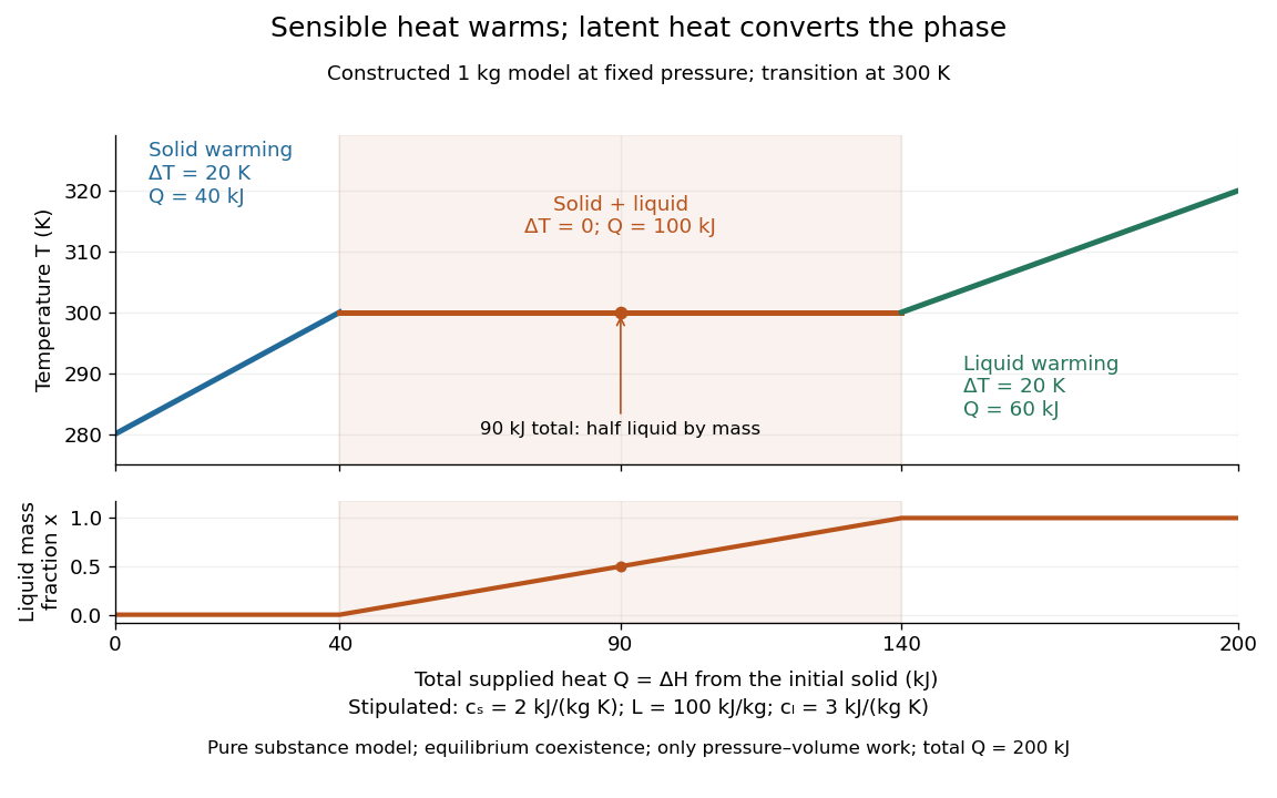
A continuous phase transition has no latent heat. Its heat capacity can have a jump or a singularity without a finite interval in which added heat converts coexisting thermodynamic phases at a constant temperature. A heating plateau therefore requires the stated phase coexistence conditions; it is not a feature of every phase transition. ^[ref]

At a first-order phase transition, the Gibbs free energy is continuous while at least one first derivative, such as entropy or volume, jumps. A nonzero entropy jump produces latent heat $L=T\Delta S$.

A phase diagram partitions a space of thermodynamic variables into regions occupied by different equilibrium thermodynamic phases and records the phase coexistence curves between them. For a pure, one-component substance, a pressure–temperature phase diagram gives one point for each pair $(T,p)$. In a single-thermodynamic phase region both controls can vary independently. On a two-thermodynamic phase phase coexistence curve, they obey one relation; at a triple point, both are fixed. These statements assume bulk thermodynamic equilibrium, fixed composition and no additional applied fields.^[ref]

At fixed temperature and pressure, the stable bulk thermodynamic phase minimizes Gibbs free energy for a fixed amount of substance. For a pure substance this is a comparison of chemical potentials on a common normalization. Two candidate thermodynamic phases coexist where ${\mu }_{\alpha }(T,p)={\mu }_{\beta }(T,p)$ and neither is exceeded in stability by a third thermodynamic phase. Differentiating their equality gives the Clapeyron equation. Thus a phase coexistence curve is a locus of equal stability, rather than a trajectory that every heated sample must follow.^[ref]

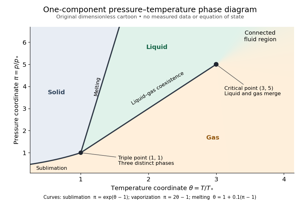
The following original cartoon uses dimensionless positive coordinates $\theta =T/T_{\ast }$ and $\pi =p/p_{\ast }$, with arbitrary reference scales $T_{\ast },p_{\ast }$. It represents no particular substance and contains no measured data. Stipulate a triple point at $(1,1)$, a liquid-gas critical point at $(3,5)$, and these drawing rules:They specify sublimation, liquid–gas phase coexistence and melting boundaries for the picture. They are not an equation of state, do not predict latent heat or mass density, and do not supply a quantitative critical theory. In particular, the melting slope is merely an illustrative choice.

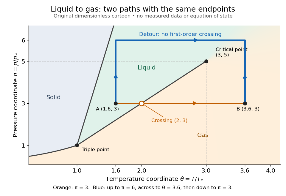
For example, at fixed $\pi =3$ the melting boundary is at $\theta =1.2$ and the liquid–gas boundary is at $\theta =2$. Heating from $(\theta ,\pi )=(1.6,3)$ to $(3.6,3)$ therefore starts in liquid, crosses phase coexistence at $(2,3)$, and ends in gas. In an equilibrium conversion at that crossing, added heat can change the phase fraction at fixed temperature through latent heat. The pressure–temperature point alone does not specify how much of each thermodynamic phase is present: for that one needs an additional amount or volume constraint.

Now connect exactly the same endpoints by raising $\pi$ from $3$ to $6$ at $\theta =1.6$, moving to $\theta =3.6$ at $\pi =6$, then lowering $\pi$ to $3$. The first leg stays on the liquid side because ${\theta }_{\mathrm{melt}}$ ranges only from $1.2$ to $1.5$ and ${\pi }_{\mathrm{vap}}(1.6)=2.2<3$. The second leg lies above the entire liquid–gas boundary, whose largest drawn pressure coordinate is $5$; the third lies beyond its largest temperature coordinate, $3$. No leg crosses a first-order phase transition boundary. The middle leg passes through a supercritical fluid region, with $\theta >3$ and $\pi >5$, and the final leg returns to a gaslike state continuously.

Avoiding a first-order phase transition does not mean that no heat or work is exchanged. Along the detour, mass density, enthalpy and heat capacity may change substantially but continuously. The liquid-gas critical point itself has singular behavior, so the detour goes around it rather than through it. This connected fluid region is the striking lesson of a phase diagram: a familiar change from liquid to gas need not involve boiling across a sharp boundary.

An equilibrium phase diagram also does not predict how rapidly a conversion occurs. Metastability and a barrier described by classical nucleation theory can delay the observed phase transition. Nor should a binary-composition phase diagram be read as the same picture: its coexistence regions and lever rule encode composition and phase fractions, and can occupy an area even though pure-substance two-thermodynamic phase coexistence occupies a curve in the pressure–temperature plane.

A truncated Perron integral over $c-iT$ to $c+iT$ recovers a summatory function with an error controlled by