
This applies normalization of an algebraic curve to the two local branches of a node.
A unit normal is a normal vector of Euclidean norm one. Given a nonzero normal vector , normalization gives . This makes a dot product measure the signed length of the normal component, without an extra factor from the length of . On a hypersurface, the two opposite choices and correspond to opposite normal orientations; a continuous choice on an orientable surface fixes its orientation of a surface.
A closed subset of a normal space is a countable intersection of open sets exactly when it is the zero set of some continuous function .
A weak shock has a small relative pressure jump. Its density jump agrees with the reversible adiabatic prediction through second order in the pressure jump, while entropy production first appears at third order.
These are the Rankine-Hugoniot conditions specialized to the mass, momentum and energy fluxes of a perfect gas.
The shock frame is an inertial reference frame in which the shock is stationary. A travelling shock then becomes a steady flow through a fixed discontinuity.
Under finite moments and a nonsingular limiting design moment, laws of large numbers make least-squares estimators converge to the true coefficient.
Least-squares differentiation gives , or its precision-weighted analogue.
Weighted least squares minimizes ; inverse-variance weights give the efficient estimator under known heteroscedasticity.
Among linear unbiased estimators in a homoscedastic linear model, least squares has minimum variance.
For a linear regression design matrix with full column rank, the ordinary least squares coefficient vector is . In a normal linear model with error covariance matrix , it is an unbiased estimator with covariance matrix . Replacing by the residual variance estimate gives the reported coefficient standard errors.
Multicollinearity means that predictor columns are strongly linearly related. It inflates coefficient variances and can make individual effects imprecise even when a joint test strongly rejects that all corresponding coefficients vanish.
The hat matrixis the orthogonal projection onto the column space of a full-rank design matrix, and the fitted response is .
Linear regression models a response's conditional expectation as a linear combination of specified predictors. In matrix form,where the design matrix describes the observations, contains the regression coefficients, and contains the errors. The fitted values estimate the response means. The model is linear in its regression coefficients; its columns may include powers, interactions, or other transformed predictors, so polynomial regression can fit curved relationships using the same machinery.
For a concrete example, take five constructed observationsAn ordinary least squares fit with an intercept gives the line . Its regression residuals are and its residual sum of squares is . A one-unit increase in the predictor corresponds to a one-unit increase in the fitted response. This is a description of this fitted association; interpreting a change as a causal effect requires the assumptions of a causal inference problem.
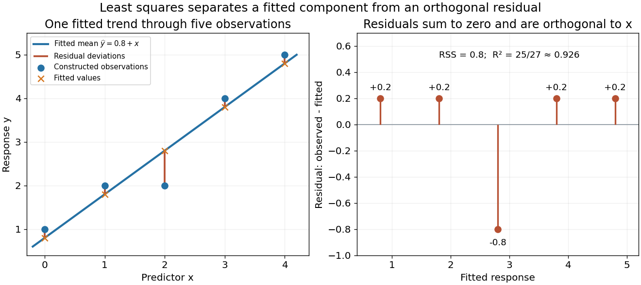
A five-point least-squares fit separates the fitted trend from residual deviations
. Details. 
The geometric reason for the fit is simple. The possible mean vectors form the column space of . Ordinary least squares chooses the orthogonal projection of the data vector onto that vector subspace, so the remaining regression residual is orthogonal to every permitted fitted direction. The least-squares normal equations express this orthogonality as . The data's explained component and unexplained component are therefore separated by the same geometry used in a Hilbert space.
The optimization definition makes sense for any observed data. Quantifying the uncertainty of the regression coefficients needs additional assumptions about the sampling and errors. With fixed of full column rank and mean-zero errors with covariance matrix , ordinary least squares is unbiased and has covariance ; the Gauss-Markov theorem compares it with other linear unbiased estimators. A normal linear model additionally makes Student t-distribution intervals and tests exact in finite samples. Model adequacy and predictive assessment remain relevant even when these calculations are available.
Two historical settings help explain the subject's appeal. Adrien-Marie Legendre's Nouvelles méthodes pour la détermination des orbites des comètes (1805) includes an appendix on the method of least squares: observations give more equations than unknowns, and squared errors provide a criterion for reconciling them. Its astronomical setting shows the motivation for combining imperfect measurements. [ref]
https://www.e-rara.ch/zut/content/titleinfo/10838079. Legendre, Nouvelles méthodes pour la détermination des orbites des comètes, 1805, appendix pp. 72–80
Francis Galton's Regression Towards Mediocrity in Hereditary Stature (1886) examines the association between parental and offspring heights and the tendency of group averages toward the population average. This is a historical use of the regression name; the modern linear model is a general statistical formulation. [ref]https://zenodo.org/records/1449548. Galton, Regression Towards Mediocrity in Hereditary Stature, 1886, original article
There are unlisted articles, also show them or only show them.