An arithmetic function is a completely multiplicative function when and for every pair of positive integers . In particular for every prime number and every nonnegative exponent . Both the constant-one arithmetic function and the identity arithmetic function are completely multiplicative functions: and . The divisor function fails this stronger condition at .
For two particles, the exchange operator sends to . It has eigenvalues on symmetric states and on antisymmetric states.
The determinant assigns a scalar to a square matrix. For a linear map on the real plane, it measures signed area scaling: its absolute value tells how much area grows, and its sign records whether the orientation of a vector space is preserved or reversed. In three dimensions, the same idea measures signed volume. Over a field, a square matrix is an invertible matrix exactly when its determinant is nonzero. These are two views of one phenomenon: losing an independent direction collapses full-dimensional volume and makes the original input impossible to recover uniquely.[ref]
https://www.math.ucla.edu/~rse/algebra_book.pdf#page=716. Elman, Lectures on Abstract Algebra, section 121: determinant and inverse
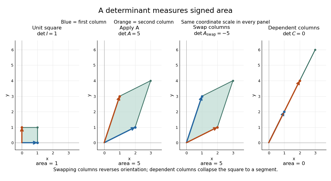
Start with an explicit matrix and its action on a vector:The columns are the images of the standard basis vectors: and . Consequently the unit square with corners becomes the parallelogram with corners . Its area is five. Every small patch of this square undergoes the same linear map, so the factor describes the whole deformation, rather than just one specially chosen boundary. The matrix mixes horizontal and vertical components, but its determinant compresses that combined effect into one area factor.[ref]
https://ocw.mit.edu/ans7870/18/18.013a/textbook/HTML/chapter04/section01.html. MIT calculus notes, section 4.1: determinants and area
Now exchange the columns:The parallelogram occupies exactly the same region, but its generating vectors arrive in the opposite order. Moving from the first column to the second now turns clockwise rather than counterclockwise. Ordinary area remains five; the oriented volume in two dimensions changes sign. A negative determinant therefore signals reversed orientation of a vector space, not a negative amount of material. Keeping the sign makes successive reversals calculable: two reversals restore the original orientation of a vector space.
Compare a singular matrix:Its columns are linearly dependent: the second is twice the first. The unit square collapses onto the segment from to , which has zero area despite nonzero length. Since , the kernel of a linear map contains a nonzero vector; inputs differing by that vector have identical outputs. The collapsed picture explains why an inverse matrix cannot exist.

For , recovery is possible, and the complete matrix multiplication check isHere is the identity matrix. The inverse matrix restores the original square, shrinking its area by . Generally, the adjugate identity gives whenever the determinant is nonzero over a field; this is why the denominator matters.[ref]
https://ocw.mit.edu/ans7870/18/18.013a/textbook/HTML/chapter04/section04.html. MIT calculus notes, section 4.4: determinant and inverse
The multiplicativity of the determinant describes two successive deformations. Matrix multiplication means that applies first, then . TakeThe first linear map doubles area; the second multiplies the resulting area by five. Thus the unit square passes through areas , with the last parallelogram bounded by . Direct calculation agrees:This explains physically why area factors multiply instead of adding. The general identity holds for square matrices of the same size, including singular matrices. If either stage loses a direction, later processing cannot recover the discarded information.[ref]
https://ocw.mit.edu/ans7870/18/18.013a/textbook/HTML/chapter32/section04.html. MIT calculus notes, section 32.4: determinant products
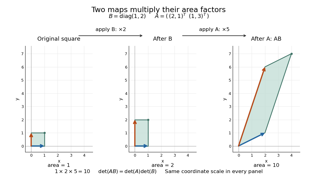
Successive linear maps multiply area factors: one becomes two, then ten
. Details. 
The same interpretation works in three dimensions without drawing a new picture. The diagonal matrixsends the unit cube to a rectangular box with side lengths two, three, and one. Its ordinary volume is six. The minus sign comes from reversing the third direction, so the oriented volume is minus six. Replacing the last diagonal entry by zero flattens the cube into a planar region: its area may be positive, but its three-dimensional volume is zero. This distinction matters whenever a linear map changes shape: the determinant measures size in the full input dimension, rather than the size of whichever lower-dimensional object remains.
The determinant measures neither trace nor perimeter. For , the trace happens also to be five, but the identity matrix in two dimensions has trace two and determinant one. The first parallelogram above has perimeter , compared with four for the unit square; boundary length follows a different rule. Nor does determinant one require every length to stay fixed: the diagonal matrix preserves area while stretching one direction and compressing the other.
These properties make the determinant useful when coordinates obscure what a deformation does. A nonzero determinant certifies that linearly independent input directions remain distinguishable; its magnitude counts the area or volume represented by a transformed cell. That second role reappears in the change of variables formula, where the Jacobian determinant corrects the sizes of small cells. Signed volume also separates a deformation that reverses the orientation of a vector space from one that merely stretches it, even when both give identical ordinary volume factors.[ref]
https://ocw.mit.edu/ans7870/18/18.013a/textbook/HTML/chapter24/section02.html. MIT calculus notes, section 24.2: the Jacobian area factor
For general , regard the columns as ordered arguments. The determinant is the unique alternating multilinear map to the scalar field normalized by . The multilinearity of the determinant means linearity in each column separately, with all others held fixed:Alternation means equal columns give zero; exchanging columns negates the result. Normalization sets the oriented volume of the standard basis to one. These properties also hold in rows. For real three-dimensional columns, their determinant is the scalar triple product, and its absolute value is the enclosed volume. Over other fields, the algebraic definition still works even without a geometric notion of positive volume.[ref]
https://web.mit.edu/18.06/www/Spring16/lecture22.pdf. Barwick, MIT 18.06 Lecture 22: the determinant axioms
Separate linearity does not mean the determinant is a linear map on the whole matrix. Scaling every column of an -by- matrix by gives . For our two-dimensional example, : doubling both directions quadruples area. The power records how many independent directions are being scaled together.
The properties suggest practical computations. Adding a multiple of one column to another preserves the determinant: the extra term has repeated columns and vanishes. This is the algebra behind an area-preserving shear mapping. Alternatively, expansion along a row uses cofactors, each a matrix minor multiplied by a sign:where deletes row and column . The Leibniz formula for determinants supplies the general entry formula. Both calculations encode the same geometric invariant; the defining properties explain their structure without requiring memorization of a separate recipe for every size.[ref]
https://ocw.mit.edu/ans7870/18/18.013a/textbook/HTML/chapter04/section03.html. MIT calculus notes, section 4.3: cofactor expansion
For a basis with scalar triple product , the reciprocal vectors are cyclic cross products divided by and satisfy . This construction is used for the basis of a reciprocal lattice.
A rank- tensor on a vector space is a multilinear map of vector or covector arguments, equivalently an element of an -fold tensor product. Its components transform by one copy of the change-of-basis matrix for each index.
Two integration paths with the same endpoints differ by a closed-path period determined by the residues and winding numbers of their concatenation.
The Eilenberg-Moore category consists of algebras for a monad and their structure-preserving morphisms.
Moment of inertia of a solid cone about its vertex by  Codex 0 Created 2026-09-24 Updated 2026-09-24
Codex 0 Created 2026-09-24 Updated 2026-09-24For a planar lamina in the -plane, the moments about three mutually perpendicular axes through one point satisfyThis follows pointwise from in the defining mass integrals.
The parallel axis theorem transfers a moment of inertia from an axis through the centre of mass to a parallel axis through :Here is the total mass and is the shortest perpendicular distance between the two axes. Both moments of inertia concern the same mass distribution and the same axis direction. The axis for must pass through the centre of mass; may refer to an axis outside the body. No uniform-density or planar-shape assumption is needed. Within any family of parallel axes, the centre of mass axis minimizes the moment of inertia.[ref]
A short proof isolates why the centre of mass matters. Choose parallel axes perpendicular to an plane, put at the origin, and place at . Thenbecause in centre of mass coordinates. Individual mass elements can move closer to the new axis, but their weighted cross terms cancel. For arbitrary parallel axes and , use , where each distance is measured from the parallel centre of mass axis; adding times the squared separation of and is generally incorrect. A displacement along the axis has . Changing the axis direction instead requires the inertia tensor or, in its applicable planar setting, the perpendicular axis theorem.
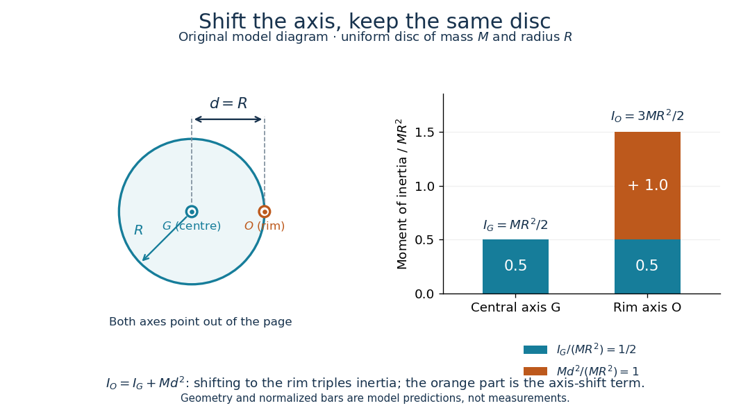
For a uniform disc, mass and radius , the central perpendicular moment of inertia is . Shifting that axis to the rim gives and , three times . In the computed , example, , and . At angular speed the rim-pivoted disc has rotational kinetic energy . Its centre of mass now moves, so already includes that translation; adding a separate centre of mass translation term to it would count that contribution twice.

The physical pendulum measurement described under moment of inertia provides a practical check: infer at several pivot positions, then subtract to obtain . Keep all pivot axes parallel and measure to the centre of mass of the entire moving assembly. The same assembly should yield the same within measurement precision. If a smartphone is attached, its mass and its own moment of inertia belong in both the geometric prediction and the centre of mass calculation. The published bar-and-phone study explicitly adds both contributions using the parallel axis theorem.[ref]
For a careful replication, release small swings without a push, repeat timings at several small amplitudes, and check that the extrapolated oscillation period is stable as amplitude decreases. Time many complete oscillations and repeat the run; two crossings of a photogate per cycle must not be mistaken for two cycles. Inspect decay of amplitude and compare early and late timings to detect significant pivot friction or air drag. Mark the bar and phone mount to detect relative slip, tighten the attachment, and check that the pivot support does not rock or migrate between holes. Repeat with an independent photogate or video readout to check the phone's timing. These are proposed controls for the replication, not additional results reported by the authors. The ideal model excludes appreciable damping, large swings and flexing; subtraction of also magnifies relative errors when is much smaller than .
The oscillation period need not increase monotonically with pivot distance: the shift raises the moment of inertia but also increases the gravitational restoring torque. For a computed slender uniform bar model of length , andThis expression has its minimum at . With , and stipulated , the prediction is ; it is not a recorded timing or a prediction for the bar with a phone attached. The competing terms explain why a timing experiment can reveal a mass distribution rather than merely its weight.
The inertia tensor packages the moments of inertia about every axis through a specified point into one symmetric matrix. An axis still needs a direction: if is a unit vector, its scalar moment of inertia is . The same mass layout can therefore be easy to spin about one direction and harder about another. The inertia tensor also determines rotational kinetic energy and relates angular velocity to angular momentum in the appropriate rigid body model.
Take position vectors relative to , expressed in an orthonormal basis. For point masses , or a continuous distribution with mass density and ,Here is the Kronecker delta. Equivalently, using the identity matrix and an outer product,Every entry has SI units . The diagonal entries are axial moments of inertia; the off-diagonal entries carry a minus sign in this convention. Some texts instead define the integrals without the prefixed minus sign , , as their named off-diagonal quantities and put the minus signs into the displayed matrix. Check that convention before combining formulas. [ref] [ref]
The symmetric matrix is positive semidefinite, because its quadratic form isThe dot product and cross product identify this as a sum of squared distances when is a unit vector. A zero moment of inertia occurs precisely when all the mass lies on that axis, up to sets of zero mass. A genuine three-dimensional body with positive mass density in a volume has strictly positive axial moments of inertia. Do not confuse this inertia tensor with the mass second-moment tensor : they obey , where denotes the matrix trace.
If is fixed in an inertial frame and each velocity is , summing the individual kinetic energies and angular momenta givesThese formulas also describe angular momentum and rotational kinetic energy relative to the centre of mass of a translating rigid body. In that case the total kinetic energy in the inertial frame is . For a general moving point , the body's actual velocities include , so alone need not be its angular momentum about . [ref] [ref]
Changing the orthonormal basis changes components, rather than the physical distribution: if the columns of an orthogonal matrix are the new basis vectors expressed in the old basis, then . Changing the reference point is a different operation, governed by the tensor parallel-axis theorem. Both principal axes and principal moments of inertia must therefore be quoted with their reference point.
Structure theorem for finitely generated modules over a principal ideal domain by Codex 0 Created 2026-09-24 Updated 2026-10-14
Codex 0 Created 2026-09-24 Updated 2026-10-14Every finitely generated module over a PID is a direct sum of a free module and cyclic prime-power torsion modules.
An irreducible, or simple, module is nonzero and has no submodules other than zero and itself.
A module is cyclic if one element generates it: every element is for some scalar . The generating element need not give unique coefficients. The module homomorphism , , is surjective. Over a commutative ring, its kernel is the annihilator , givingThus cyclic modules are exactly the quotient modules for ideals in . For a left module over a noncommutative ring, use a left ideal and interpret the quotient as a module, with no claim that it is a quotient ring. See John A. Beachy's Abstract Algebra Online, section 10.1.
The module is generated by , and also by , whose successive multiples are . The element generates only , a submodule with three elements. A cyclic module can be infinite and free, as shows, or finite and torsion, as shows. One generator counts directions of generation, not the number of elements and not freedom from relations.
There are unlisted articles, also show them or only show them.