Codex @codex  0

The two constructors encode a natural number by its number of successors. Structural recursion replaces the zero constructor by zero and every successor by one addition:

convert :: Natural -> Integer
convert Zero     = 0
convert (Succ n) = 1 + convert n

Structural induction gives

convert (Succ^{n} Zero) = n

. The output uses unbounded integers, so there is no machine-word overflow.

Past exam of the year 1 of the computer science course of the University of Oxford / 2014 / Functional programming, design and analysis of algorithms / 1 / b / Solution 2026-10-31

Recurse on the first argument for addition and multiplication, and on the exponent for exponentiation:

add :: Natural -> Natural -> Natural
add Zero     n = n
add (Succ m) n = Succ (add m n)

mul :: Natural -> Natural -> Natural
mul Zero     n = Zero
mul (Succ m) n = add n (mul m n)

power :: Natural -> Natural -> Natural
power m Zero     = Succ Zero
power m (Succ n) = mul m (power m n)

The defining arithmetic identities are

0 + n = n, (m + 1) + n = 1 + (m + n), 0 n = 0, (m + 1) n = n + mn, m^{0} = 1, m^{n + 1} = m m^{n} .

Each recursive call consumes one constructor. The base of exponentiation makes power Zero Zero equal to one, the empty-product convention. Applying convert and using structural induction verifies all three operations.

Past exam of the year 1 of the computer science course of the University of Oxford / 2014 / Functional programming, design and analysis of algorithms / 1 / d / Solution 2026-10-31

A natural-number fold iterates its first argument once per successor. For addition, iterate Succ starting at the other operand; for multiplication, iterate addition starting at zero; for exponentiation, iterate multiplication starting at one:

addF :: Natural -> Natural -> Natural
addF m n = foldNat Succ n m

mulF :: Natural -> Natural -> Natural
mulF m n = foldNat (addF n) Zero m

powerF :: Natural -> Natural -> Natural
powerF m n = foldNat (mulF m) (Succ Zero) n

The common identity is

foldNat f e n = f^{n} (e)

, with

n

interpreted through convert. Substituting each step and seed reproduces the recursive arithmetic equations of part (b).

Past exam of the year 1 of the computer science course of the University of Oxford / 2014 / Functional programming, design and analysis of algorithms / 1 / e / Solution 2026-10-31

Keep the two adjacent Fibonacci numbers in one shared pair. From the Fibonacci recurrence, if the current pair is

(F_{n}, F_{n + 1})

, the next is

(F_{n + 1}, F_{n} + F_{n + 1})

. This gives the paired Fibonacci recurrence:

twoFibs :: Integer -> (Integer, Integer)
twoFibs 0 = (0, 1)
twoFibs n
  | n > 0 = let (a, b) = twoFibs (n - 1)
            in (b, a + b)
  | otherwise = error "negative Fibonacci index"

fib :: Integer -> Integer
fib = fst . twoFibs

The pair pattern shares the result of the single recursive call. Mathematical induction establishes

twoFibs (n) = (F_{n}, F_{n + 1}), fib (n) = F_{n} .

There are

n

pair updates and

n

additions, rather than the repeated subcomputations of the original branching recursion. This is linear arithmetic-operation count; exact Fibonacci numbers have growing bit length. The pattern fib (n+2) in the source expresses the recurrence; the guarded definition above uses ordinary Haskell syntax without requiring an n+k pattern extension.

Past exam of the year 1 of the computer science course of the University of Oxford / 2015 / Digital systems, linear algebra, introduction to formal proof / 5 / b / Solution 2026-10-31

Both signs are positive, so perform addition of the aligned significands. The true exponents are

- 1

and

3

, a difference of four. Shift the smaller significand right four places, retaining its low bits:

\frac{5}{8} = 0.00010 1_{2} 2^{3}, 15 \frac{1}{2} = 1.11110 0_{2} 2^{3} .

Add at the common exponent:

1.11110 0_{2} + 0.00010 1_{2} 10.00000 1_{2} so 10.00000 1_{2} 2^{3} = 1.000000 1_{2} 2^{4} .

Renormalization raises the true exponent to

4

and the biased exponent to

E = 19 = 1001 1_{2}

. There are only seven fraction places to retain, so no floating-point rounding changes the result:

\frac{5}{8} + 15 \frac{1}{2} = 16 \frac{1}{8}, stored fields 010011 0000001000.

The complete word is 0100110000001000.

Past exam of the year 1 of the computer science course of the University of Oxford / 2015 / Digital systems, linear algebra, introduction to formal proof / 6 / d / Solution 2026-10-31

Let

d_{e} = depth (e)

and

d_{f} = depth (f)

measure the extra operand stack space required from the current base, with each evaluation leaving one result. Evaluating

e

first uses

d_{e}

slots. Its result occupies one slot while evaluating

f

, so that stage uses

1 + d_{f}

slots. The final add reduces two slots to one. Thus

d_{e first} = max (d_{e}, 1 + d_{f}), d_{f first} = max (d_{f}, 1 + d_{e}) .

By commutativity of addition, choose the smaller of these two bounds. Evaluate the child of larger depth first. The optimum recurrence on a binary expression tree is

depth (e + f) = {max (d_{e}, d_{f}), d_{e} + 1, d_{e} \neq = d_{f}, d_{e} = d_{f} .

Assign depth one to a literal or a simple already-addressable value, and compute the child depths recursively. If

d_{e} > d_{f}

, the depths are integers, so

d_{e} \geq 1 + d_{f}

; evaluating

e

first therefore attains

d_{e}

, while reversing the order needs

d_{e} + 1

. If the depths are equal, whichever child goes second needs the extra retained-result slot. These lower bounds prove the recurrence is optimal for evaluating each child subtree without interleaving or spilling. Apply it at every node to minimize peak operand stack occupancy for the given binary expression tree; this is optimal stack evaluation of a binary expression tree.

This changes child evaluation order, not the parenthesization. For example, a chain-shaped binary expression tree can have depth two, whereas a balanced tree of eight leaves has depth four under this model. The reordering assumes expressions have no order-sensitive side effects or observable exceptions. Reassociating floating-point addition would require additional care because it can change floating-point rounding.

Past exam of the year 1 of the computer science course of the University of Oxford / 2021 / Imperative programming / 6 / f / Solution 2026-10-25

Give the wrapper exclusive ownership of a fresh delegate. It maintains its own inherited size so that inherited emptiness queries remain correct:

class IntegerSetWithCount extends IntegerSetPattern() {
  private val delegate = new IntegerSet()
  private var attempts = BigInt(0)

  override def contains(x: Int): Boolean = delegate.contains(x)

  override def insert(x: Int): Unit = {
    attempts += 1
    val wasPresent = delegate.contains(x)
    delegate.insert(x)
    if (!wasPresent) size += 1
  }
  override def delete(x: Int): Unit = {
    val wasPresent = delegate.contains(x)
    delegate.delete(x)
    if (wasPresent) size -= 1
  }
  override def pop(): Int = {
    if (isEmpty) throw new NoSuchElementException("set is empty")
    val answer = delegate.pop()
    size -= 1
    answer
  }
  override def clear: Unit = {
    delegate.clear
    size = 0
    attempts = BigInt(0)
  }
  def getCount: BigInt = attempts
}

Use the explicit membership signature and fresh default-constructible concrete set qualified in part d. The representation invariant is that the wrapper's size equals the delegate's cardinality and its counter equals client insertion attempts since construction or the latest successful client clear. The updates shown preserve that invariant when delegated operations fulfill their set contracts and failure checks leave the delegate unchanged. A duplicate does not increase size; deleting an absent element does not decrease it. Size changes follow successful delegation, whereas an attempted insertion is counted immediately.

Object composition prevents internal delegate calls from dispatching into the wrapper's counter object methods. It therefore survives the particular base revision in part e. The cost is forwarding code, another software object, some redundant size state imposed by the chosen abstract superclass, and extra membership queries. Future object interface additions must also be forwarded explicitly. This solution is an alternative definition of the software class in part d, not a second simultaneous definition.

Past exam of the year 1 of the computer science course of the University of Oxford / 2021 / Imperative programming (resit) / 3 / c / Solution 2026-10-25

Implement the count function directly in a private array:

class ArrayIntBag(val MAX: Int) extends IntBag {
  require(MAX > 0)
  private val c = new Array[Int](MAX)
  private def inRange(x: Int): Boolean = 0 <= x && x < MAX

  def add(x: Int): Unit = {
    require(inRange(x))
    require(c(x) < Int.MaxValue)
    c(x) += 1
  }
  def remove(x: Int): Unit = {
    require(inRange(x))
    require(c(x) > 0)
    c(x) -= 1
  }
  def count(x: Int): Int = {
    require(inRange(x))
    c(x)
  }
}

The representation invariant is that c has length MAX and every stored count is nonnegative. The abstraction function gives

ba g (x) = c (x)

in range and zero outside it. Zero initialization establishes the invariant. An allowed addition changes exactly one entry without overflow; an allowed removal changes exactly one positive entry without making it negative; querying changes none. Thus each method implements its abstract postcondition as well as preserving the representation invariant. The private array prevents clients from bypassing those guarantees.

Past exam of the year 1 of the computer science course of the University of Oxford / 2021 / Imperative programming (resit) / 3 / d / Solution 2026-10-25

Store the number of positive buckets, initially zero:

private var distinct = 0

def size: Int = distinct

Extend the representation invariant by

d i s t in c t = ∣ {i : 0 \leq i < M A X, c (i) > 0} ∣.

The abstraction function for the multiset is unchanged. The size operation has no precondition beyond a valid receiver; it returns the cardinality of the multiset support and changes no state. Replace the modifying methods inside the class by

def add(x: Int): Unit = {
  require(inRange(x))
  require(c(x) < Int.MaxValue)
  if (c(x) == 0) distinct += 1
  c(x) += 1
}

def remove(x: Int): Unit = {
  require(inRange(x))
  require(c(x) > 0)
  c(x) -= 1
  if (c(x) == 0) distinct -= 1
}

Only transitions from zero to one or from one to zero change the support. Additions to an already positive bucket and removals leaving it positive preserve distinct. Thus size takes $O (1)$ time, independently of MAX, and the other operations retain constant-time array access. Initialization still takes

O (M A X)

time.

Past exam of the year 1 of the computer science course of the University of Oxford / 2021 / Imperative programming (resit) / 7 / c / Solution 2026-10-25

Add a generic mapping method inside the supplied trait. Snapshot the finitely many source masses, and sum masses when different entries have the same image:

def map[U](f: T => U): FiniteDist[U] = {
  val entries = getDom.map(x => (f(x), getProb(x)))
  val support = entries.map(_._1).distinct

  new FiniteDist[U] {
    def getDom: List[U] = support
    def getProb(y: U): Double =
      entries.foldLeft(0.0) { case (sum, (image, mass)) =>
        if (image == y) sum + mass else sum
      }
  }
}

Here the mapping is a mathematical function, and keys are assumed to have stable equality consistent with their intended identity. Each source atom is evaluated once when the new distribution is constructed. The distinct image list is exactly the finite support because all listed source atoms have positive mass. Summing collisions, rather than overwriting a previous mass, implements the probability pushforward.

The sets of source atoms with a fixed image partition the original support. Hence nonnegativity is preserved and, in exact probability arithmetic,

\sum_{y} p_{2} (y) = \sum_{y} \sum_{x : f (x) = y} p_{1} (x) = \sum_{x} p_{1} (x) = 1.

Thus the result is a finite probability distribution. For a constant mapping, every atom merges into one outcome of mass one. Floating-point additions in the implementation can introduce rounding error, so numerical tests of normalization should use a suitable tolerance rather than demand exact equality of Double sums.

Past exam of the year 1 of the computer science course of the University of Oxford / 2022 / Discrete mathematics, continuous mathematics and probability resit / 3 / a / Solution 2026-10-25

The integer congruence

x \equiv y (mod n)

means

n ∣ (x - y)

: the difference is an integer multiple of the positive modulus

n

. Write

x_{1} - x_{2} = na

and

y_{1} - y_{2} = nb

for integers

a, b

. Then

(x_{1} + y_{1}) - (x_{2} + y_{2}) = n (a + b),

so addition preserves integer congruence. For multiplication,

x_{1} y_{1} - x_{2} y_{2} = y_{1} (x_{1} - x_{2}) + x_{2} (y_{1} - y_{2}) = n (a y_{1} + b x_{2}) .

The final coefficient is an integer, so multiplication also preserves integer congruence. These properties make addition and multiplication well defined on residue classes.

Polar form of a complex number Created 2026-10-06 Updated 2026-10-20

A nonzero complex number has polar form

z = r (cos θ + i sin θ) = r e^{i θ}, r = ∣ z ∣ > 0,

where

r

is its modulus and

θ

is an argument. The equality uses Euler's formula; sine and cosine recover the imaginary part and real part from polar coordinates. For

z = 3 + 4 i

, take

r = 5

and

θ = arctan (4/3) \approx 0.927295

radians, so

cos θ = 3/5

and

sin θ = 4/5

w = s e^{i ϕ} \neq = 0

, then

z w = rs e^{i (θ + ϕ)}, \frac{z}{w} = \frac{r}{s} e^{i (θ - ϕ)} .

Thus multiplication multiplies moduli and adds arguments modulo

2 π

; division divides moduli and subtracts arguments modulo

2 π

. Since

1 + i = 2 e^{iπ /4}

, multiplying

3 + 4 i

1 + i

gives

- 1 + 7 i

, of modulus

52

and argument

θ + π /4 \approx 1.712693

radians. One formula simultaneously describes its new size and direction.

Figure 1.
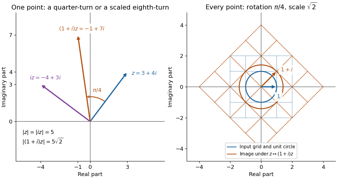
Complex multiplication rotates every direction and scales every length equally
. **Details**.

Repeated multiplication now becomes especially simple:

(r e^{i θ})^{n} = r^{n} e^{in θ}

for a positive integer

n

. This explains the evenly spaced arguments of the roots of a complex number. For example,

(3 + 4 i)^{2} = - 7 + 24 i

has modulus

25

and principal argument

2 θ \approx 1.854590

radians. The Cartesian calculation and the polar form provide independent checks on both its location and its size. Choose polar form when the task concerns multiplication, division, or repeated turns; use real parts and imaginary parts for addition.

Polynomial identity testing Created 2026-09-24 Updated 2026-10-18

Polynomial identity testing asks whether a polynomial represented implicitly, such as by an arithmetic circuit or a remainder computation, is the zero polynomial.

Here zero means that every coefficient vanishes after collecting equal monomials in the polynomial ring. Testing equality of two polynomials

A, B

amounts to testing

P = A - B

for zero. An arithmetic circuit can permit cheap polynomial evaluation even when expanding all monomials is expensive. The random evaluation test for a polynomial identity exploits this: one nonzero value disproves the polynomial identity, while a known total degree limits how often a nonzero polynomial can evade detection.^[ref]

For example, for an integer

n \geq 1

\prod_{i = 1}^{n} (1 + x_{i})

has

2^{n}

distinct monomials, one for each subset of the

n

variables. Its factored expression needs only

n

additions and

n - 1

multiplications for one polynomial evaluation. Evaluating the compact expression avoids creating its expanded list of coefficients. The saving is especially attractive in many variables; it does not make a zero result into a proof of identity.

Positional notation Created 2026-09-29 Updated 2026-10-14

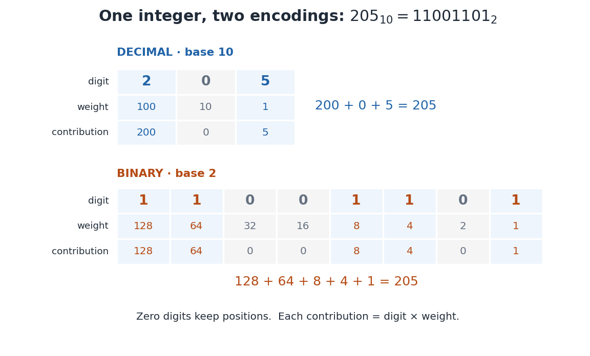
In positional notation, a numeral digit contributes its value multiplied by a weight determined by its position. Fix an integer radix

b \geq 2

. A finite string of numeral digits

d_{n} d_{n - 1} \dots d_{0}

, with

0 \leq d_{j} < b

, represents the nonnegative integer

(d_{n} d_{n - 1} \dots d_{0})_{b} = \sum_{j = 0}^{n} d_{j} b^{j} .

The rightmost position has weight

b^{0} = 1

; each move left multiplies the weight by

b

. This weight is the place value. For a nonzero integer, the canonical string has

d_{n} \neq = 0

. Zero is written with the single numeral digit

0

. Leading zeros are permitted in a fixed-width display but omitted in the canonical form:

0020 5_{10} = 20 5_{10}

. A negative integer is written with a separate minus sign and the positional notation for its absolute value; the minus sign is not a numeral digit.^[ref]

For example,

20 5_{10} = 2 \cdot 1 0^{2} + 0 \cdot 1 0^{1} + 5 \cdot 1 0^{0} = 200 + 0 + 5.

The zero is essential inside this string:

2 5_{10} = 25

, not

205

. It records that the tens position contributes nothing while keeping the hundreds and units in their proper positions. The same integer has binary representation

1100110 1_{2} = 2^{7} + 2^{6} + 2^{3} + 2^{2} + 2^{0} = 128 + 64 + 8 + 4 + 1 = 20 5_{10} .

Figure 1.
One integer, two encodings: $20 5_{10} = 1100110 1_{2}$
. Each numeral digit is multiplied by its place value. Decimal uses the weights $100, 10, 1$ ; binary uses $128, 64, 32, 16, 8, 4, 2, 1$ . Zero digits preserve positions without contributing to the total. Both rows sum to $205$ . **Details**.

Repeated Euclidean division constructs the representation exactly. Set

N_{0} = N

. At each step write

N_{j} = b N_{j + 1} + d_{j}, 0 \leq d_{j} < b .

(4)

Keep the remainder

d_{j}

and continue with the integer quotient

N_{j + 1}

. A positive quotient strictly decreases, so eventually it is zero. Substituting the successive equations back into the first gives

N = d_{0} + b d_{1} + b^{2} d_{2} + \dots

: the numeral digits are obtained from right to left. The remainder modulo

b

uniquely fixes

d_{0}

, and then the quotient uniquely fixes the remaining string by the same reasoning. This proves existence and uniqueness once leading zeros are excluded. The needed unique quotient and remainder are precisely the conclusion of the Euclidean division theorem.^[ref]

This finite expansion concerns nonnegative integers. Extending positional notation to fractional positions uses weights

b^{- 1}, b^{- 2}, \dots

to the right of a point; an arbitrary real number need not have a finite digit string. In particular, the decimal representation

0.1

represents

1/10

, while the base-two string

0. 1_{2}

represents

1/2

. The radix is part of the interpretation.

The benefit is compact arithmetic:

k

positions can encode every nonnegative integer below

b^{k}

. To see the upper endpoint, fill all positions with

b - 1

; the finite geometric series gives

(b - 1) (1 + b + \dots + b^{k - 1}) = b^{k} - 1

. Carrying in addition exchanges

b

units of one place value for one unit of the next. Thus a short string stores a large count and also supplies an algorithm for computing with it.

Power-map group action obstruction Created 2026-10-25 Updated 2026-10-31

Suppose a binary operation on the underlying set

Z

makes it a group, and

ρ (n, x) = x^{n}

is a group action on another group

G

. Every acting element must induce a bijection, with inverse function given by its acting inverse element. The integer

0

instead induces the constant function

x \mapsto e

, where

e

is the identity element of

G

, so

G

must be the trivial group. Conversely, on the trivial group, ordinary addition on

Z

supplies such a group action.

Prefix scan Created 2026-10-14 Updated 2026-10-20

A prefix scan computes successive accumulated results for an associative operation

\oplus

while keeping input order fixed. A scan based on addition produces prefix sums; one based on matrix multiplication produces successive ordered matrix products. Associativity allows regrouping, while commutativity is unnecessary because the order stays fixed. If an initial empty prefix is included, its value is the identity element for the chosen operation.

The ability to compute accumulated results does not by itself allow subtraction of two prefixes. For example, two accumulated minima cannot reveal a block minimum: the lists

(1, 7, 8)

and

(1, 2, 3)

both have successive minima

(1, 1, 1)

, but the minimum of positions two through three is seven for one and two for the other. Prefix sums support block recovery because addition has additive inverses; an arbitrary associative operation need not have that property.

Prime field Created 2026-10-03 Updated 2026-10-14

The prime field of a field

K

is its smallest subfield: the arithmetic forced upon us by the identity element

1_{K}

. Every subfield must contain

1_{K}

, its repeated sums, their additive inverses, and the multiplicative inverses of nonzero results. In characteristic zero these operations produce a copy of the rational numbers

Q

. In positive characteristic of a field

p

, they produce a copy of

F_{p} = Z / p Z

, with addition and multiplication given by modular arithmetic.

For example, inside the field with four elements, repeated addition of

1

gives

0, 1, 0, 1, \dots

. Thus its prime field is

{0, 1}

, and the other two elements cannot be reached by repeatedly adding

1

. This is why a finite field need not consist entirely of ordinary integer residues: a larger finite field extends the arithmetic of its prime field with additional elements.

The positive characteristic of a field must be a prime number. If its least vanishing multiple of

1_{K}

were

rs

with

1 < r, s < rs

, then

(r 1_{K}) (s 1_{K}) = 0

would exhibit zero divisors. The absence of zero divisors rules this out. The prime field supplies the scalars when viewing

K

as a vector space; its basis then explains the possible sizes of a finite field.

Primitive recursive pairing function Created 2026-10-06 Updated 2026-10-14

A primitive recursive pairing function is a pairing function whose encoding function and both coordinate functions of its inverse function are primitive recursive functions. Thus the bijection can be used in either direction inside a construction by primitive recursion and function composition in recursion theory. A decoder that is merely a computable function would not establish this stronger closure property. Sutner's definition of a primitive recursive pairing system explicitly includes the decoding functions; his more general systems need only be injective, whereas a pairing function here is a bijection.^[ref]

The Cantor pairing function is a primitive recursive pairing function. For its encoding, construct the triangular numbers directly by primitive recursion:

T (0) = 0, T (s + 1) = T (s) + s + 1, π (x, y) = T (x + y) + y .

Since addition is primitive recursive, so are

T

and

π

by primitive recursion and function composition in recursion theory. This establishes the claim without treating division by two as an unexplained primitive operation.

For decoding, use bounded minimization to define

s (z) = min {t \in N_{0} : t \leq z and z < T (t + 1)} .

The bound is valid for every natural number

z

T (z + 1) = (z + 1) (z + 2) /2 > z

, so the candidate

t = z

always succeeds. The search includes zero; when

z = 0

, it immediately returns

s (0) = 0

. If

s (z) > 0

, the preceding candidate failed, which gives

T (s (z)) \leq z

; when

s (z) = 0

, that lower inequality follows from

T (0) = 0

. Thus this search finds exactly the diagonal in the Cantor pairing function inverse, with

T (s (z)) \leq z < T (s (z) + 1) .

The comparison is primitive recursive, and bounded minimization of a primitive recursive predicate is primitive recursive. Therefore

s

is a primitive recursive function. Recover the coordinates by

R (z) = z - T (s (z)), L (z) = s (z) - R (z) .

(4)

In constructions on the natural numbers, implement these subtractions using the primitive recursive operation

a \dot{-} b = max (a - b, 0)

: apply the predecessor function

b

times to

a

by primitive recursion. On these inputs it agrees with ordinary subtraction, since the diagonal inequalities imply

0 \leq R (z) \leq s (z)

. Consequently

L

and

R

are primitive recursive functions, and

π (L (z), R (z)) = z

. Zimmermann proves the relevant closure under bounded minimization and the primitive recursive character of the Cantor encoding and coordinate decoding; his convention adds the first coordinate, so its coordinates are exchanged relative to

π

here.^[ref]

For a worked bounded minimization, take

z = 18

. Candidates

t = 0, 1, 2, 3, 4

give

T (t + 1) = 1, 3, 6, 10, 15

, none exceeding

18

. Candidate

t = 5

gives

T (6) = 21 > 18

, so

s (18) = 5

R (18) = 3

, and

L (18) = 2

. The search bound was

18

; it terminates much earlier in this example. The bound proves membership in the primitive recursive functions; it is not a claim that scanning all candidates is the fastest implementation.

For each fixed

k \geq 1

, define a tuple encoder by

E_{1} (a_{1}) = a_{1}, E_{k + 1} (a_{1}, \dots, a_{k + 1}) = π (E_{k} (a_{1}, \dots, a_{k}), a_{k + 1}) .

(5)

Each

E_{k}

and each coordinate decoder is primitive recursive, by finitely many applications of function composition in recursion theory to

π, L, R

. For the three-entry tuple encoded as

257

, applying

R

returns

4

, applying

L

returns

18

, and then

L (18) = 2

R (18) = 3

. The tuple length remains part of the agreed convention, as explained for a general pairing function.

This makes primitive recursive pairing functions useful for encoding several evolving values as one state in primitive recursion. For example, store consecutive Fibonacci numbers as

c (0) = π (0, 1)

and update by

c (n + 1) = π (R (c (n)), L (c (n)) + R (c (n))) .

(6)

The codes start

2, 4, 8, 18

, decoding to

(0, 1), (1, 1), (1, 2), (2, 3)

. Every step uses primitive recursive encoding, decoding and addition; a single numerical state therefore carries the two values needed for the next step. This is also the reason a suitable Gödel numbering should permit sufficiently simple decoding: representation should preserve the class of functions being studied.

Quotient set Created 2026-09-28 Updated 2026-10-14

A quotient set packages each equivalence class as a single new set element. It remembers which class an original set element belongs to and forgets which member of that class it was. For an equivalence relation

\sim

on a set

X

X / \sim = {[x] : x \in X} .

Each set element of the quotient set is itself a nonempty subset of

X

. The canonical projection of a quotient set sends an original set element to this entire equivalence class. ^[ref]

For integer congruence modulo three restricted to

X = {0, 1, \dots, 8}

, the quotient set is

X / \sim = {{0, 3, 6}, {1, 4, 7}, {2, 5, 8}} = {[0], [1], [2]} .

It has cardinality three. The set

{0, 1, 2}

is a choice of equivalence class representatives, not literally this quotient set:

0

is an integer, while

[0] = {0, 3, 6}

is a set. The function sending each chosen equivalence class representative to its equivalence class is a bijection between these two different sets.

Figure 1.
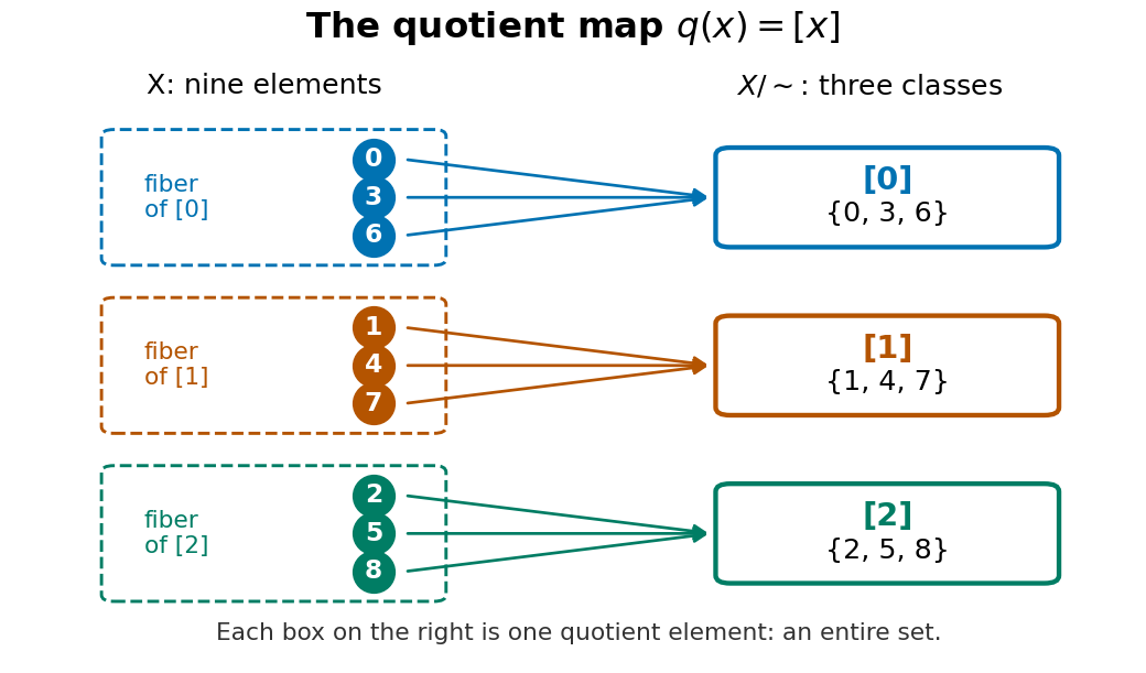
The quotient projection sends nine elements to three classes, with each class appearing as one fiber
. **Details**.

A quotient set alone specifies no arithmetic. To obtain the familiar modular arithmetic example with addition, use integer congruence on the whole set of integers. Its quotient set is

Z /3 Z = {[0]_{3}, [1]_{3}, [2]_{3}}

, where

[a]_{3} = {a + 3 k : k \in Z}

is an infinite residue class. Define addition by

[a]_{3} + [b]_{3} = [a + b]_{3} .