Luis Walter Alvarez's program extended the Glaser bubble-chamber experiment into large hydrogen bubble chambers and systematic analysis. His lecture credits John G. Wood, an accelerator technician, with early hydrogen tracks, and emphasizes technicians' responsibility for chamber development.[ref]
Recent Developments in Particle Physics by Luis Walter Alvarez. Recent Developments in Particle Physics, lecture 11 December 1968; institutional report UCRL-18696, printed pp. 12–16, Fig. 2
Alvarez's 1956 report describes a ten-inch hydrogen bubble chamber in a steady magnetic field, exposed to a negative-pion beam for proton scattering. Liquid hydrogen was the target. Horizontal windows admitted illumination and stereo viewing; a shielded light source let bubble-scattered light reach the lenses. A temperature gradient initially restricted sensitivity near the top. Tilting and fast recompression improved uniformity.[ref]
Liquid Hydrogen Bubble Chambers by Luis Walter Alvarez. Liquid Hydrogen Bubble Chambers, UCRL-3367, 4 April 1956, PDF pp. 5–7: ten-inch chamber, optics, recompression and scattering exposure
The same report compares tracks without a magnetic field against straightness expectations, testing spurious curvature. Multiple Coulomb scattering remained a limitation. This separates an instrumental check from the physical momentum inferred with the field on.[ref]
Liquid Hydrogen Bubble Chambers by Luis Walter Alvarez. UCRL-3367, PDF p. 7, paragraph beginning “The no field tracks”
The scientific opportunity is to turn a visible geometry into a test of an invisible intermediate state. The bubble-chamber pressure cycle prepares the sensitive target; bubble-chamber track readout supplies geometric measurements. Neither step alone identifies a particle resonance.
Stereoscopy supplies depth because different cameras see different projections of the same track. A functional reconstruction first matches the same interaction vertex and track segments across views. A calibrated lens and window model maps each measured image coordinate back to a ray inside the liquid. Refraction at the windows must be included. Intersecting the rays, or finding their closest agreement when measurements have errors, estimates three-dimensional coordinates. Several points then determine a trajectory, rather than only a projected arc.
An original ideal-camera model makes the geometry explicit. Take two parallel pinhole cameras with centers and , focal length , and optical axes along . Use virtual image planes in front of the pinholes so that image coordinates have the same orientation as the scene. A point then givesSubtracting the horizontal image coordinates gives disparity , henceFor stipulated , , , and , the reconstructed point is . These are ideal optical inputs, not dimensions of Alvarez's apparatus. This model omits refraction and lens distortion; actual calibration replaces its simple ray geometry. Since , the same disparity error gives worse depth precision for distant points.
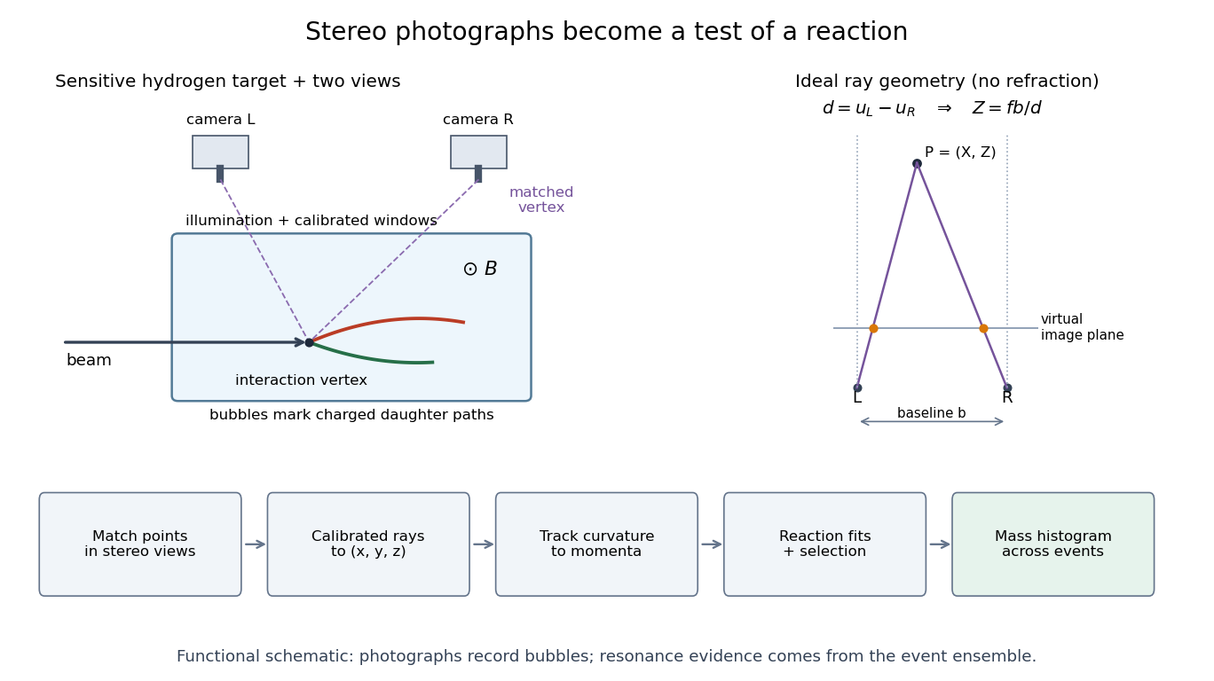
From stereo bubble photographs to coordinates, momenta and an event ensemble
. Original functional diagram. The chamber, camera positions and tracks are schematic, not a historical mechanical drawing. The parallel-camera ray construction illustrates an idealized model without refraction. Details.
The Lorentz force then supplies a momentum scale. With magnetic field uniform and negligible stopping power over a fitted segment, bubble-chamber track readout gives . The local three-dimensional helix tangent supplies the missing direction: if is its angle to the field, . In practical units,Here is the elementary charge and the speed of light. A short, almost straight arc poorly constrains its radius of curvature; a visually sharp track can therefore have poor momentum precision.
Alvarez describes a progression from measured coordinates to momenta and angles, then conservation-constrained fits testing alternative track identities. Computer programs made the repeated tests practical; an insufficiently constrained event could retain several hypotheses.[ref]
Recent Developments in Particle Physics by Luis Walter Alvarez. UCRL-18696, printed pp. 30–33: HYDRO, PANG, GUTS, KICK and SUMX
A mathematical formulation explains what such a fit can establish. Let collect measured momenta and angles, with positive-definite covariance matrix . For a chosen reaction hypothesis, adjust them to by minimizing a generalized least squares objective,The constraints express four-momentum conservation and any independently known daughter masses. For each proposed identity, calculate energy from the energy–momentum relation, . A missing neutral particle adds unknowns; a measured decay vertex can add geometric constraints. Compatibility depends on the measurement errors and the independent constraints, not just the smallest raw among unrelated fits.
A simple independent check uses a single momentum conservation constraint. Suppose two measured one-dimensional momenta are and , each with independent standard deviation , and a stipulated parent at rest requires their sum to vanish. Minimizing the two equal-weight squared changes gives fitted values and , with . A fit repairs a mismatch according to a hypothesis; it does not prove that hypothesis. This one-component illustration is not a complete reaction fit.
Why add the daughter four-momenta? Consider a selected combination of final particles withUsing the Minkowski metric, its scalar square isIn the combination's center-of-momentum frame, its total momentum vanishes and its total energy is . Therefore , givingLorentz transformations preserve this scalar square, so the reconstructed invariant mass does not depend on the combination's laboratory motion. It includes relative kinetic energy and need not equal the sum of the daughter rest masses. A random pair has an invariant mass too; that number does not itself establish a common parent.
For two daughters, expanding the square and substituting each energy–momentum relation givesHere and are masses, not energies. Reporting in and momenta in is equivalent to calculating numerically with and in . Setting in natural units suppresses these conversion factors; it does not change the measured quantity.
Alvarez's lecture illustrates invariant mass searches with combinations and contrasts resonance lifetimes near with the much longer lived states the chambers originally targeted. These resonances decayed before producing a resolvable parent track.[ref]
Recent Developments in Particle Physics by Luis Walter Alvarez. UCRL-18696, printed pp. 46–47, Figs. 15–17: effective-mass histograms and short lifetimes
Operationally, choose a reaction hypothesis, require an acceptable bubble-chamber kinematic fitting result, and form specified daughter combinations. Accumulate their invariant masses in a histogram across events. A particle resonance is inferred from the ensemble's dynamics; its short-lived parent is not directly photographed. Daughter tracks can be visible even when the production and decay positions of the parent cannot be separated. Wrong combinations create background, and several combinations from one event are statistically correlated.
Take two stipulated oppositely charged daughters with equal rest mass and exactly opposite momenta of magnitude . Their total momentum is zero, soThis is a constructed event, not an identification of a historical particle. Boosting both four-momenta by along the first daughter's direction gives total energy and total momentum . Substitution recovers the same invariant mass, although the laboratory energy has increased.
The following independent simulation stipulates 700 signal combinations from a Cauchy distribution centered at with scale , truncated to , plus 2400 background combinations whose density decreases linearly across that interval. Each combination is converted to a back-to-back two-daughter event with . Independent isotropic directions are chosen, each Cartesian momentum component receives normal distribution noise with standard deviation , and invariant mass is reconstructed from the perturbed momenta. All inputs and counts are invented. No historical experimental points or fitted historical parameters appear.
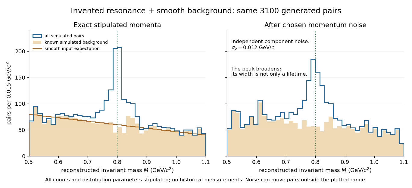
A stipulated resonance component produces an excess above a smooth simulated invariant-mass background
. Original simulation of two-daughter events, with invented counts, a truncated Cauchy signal and a linearly falling background. The two panels share the same generated events. The right panel adds chosen momentum noise before reconstructing invariant mass; this is not an experimental discovery plot. Details.
The simulation separates a stipulated physical distribution from measurement broadening. Its Cauchy distribution is only a convenient resonance-shaped input, not a complete quantum scattering model. Spatial resolution, magnetic field calibration, Multiple Coulomb scattering, stopping power and incorrect daughter identities all propagate into the measured invariant mass. Instrumental broadening must be understood before interpreting an observed width as a lifetime.
Selection also changes the shape. A momentum threshold can remove low-invariant mass pairs; a fit that fixes the candidate parent's mass would artificially concentrate that same mass and cannot supply an independent search distribution. Compare accepted simulated events with the input distribution, vary justified selection criteria, and check neighboring invariant mass intervals. A peak supported only by one untested selection is weaker evidence than a structure that survives calibration and background checks. The smooth background in the figure is a stipulated control component, not a claim that every physical background is smooth.
Articles by others on the same topic
There are currently no matching articles.