Barnett effect

The Barnett effect is the change of a body's magnetization caused by mechanical rotation. Turning the whole specimen can bias the internal angular momentum carrying its magnetic moments, even with zero applied magnetic field. It is the reciprocal physical question to the Einstein-de Haas effect: impose rotation and measure magnetization, rather than change magnetization and observe mechanical motion. The relation between the two becomes especially transparent when the same signed gyromagnetic ratio connects magnetic moment and internal angular momentum.

Samuel Jackson Barnett published Magnetization by Rotation on 1 October 1915 in Physical Review. The Barnett rotation magnetometry experiment below provides an inspected modern example. The important distinction is between an equivalent term in a Hamiltonian and the actual external magnetic field measured by a magnetometer: the first biases the material; its resulting magnetization produces the second.

Let the specimen rotate uniformly with angular velocity $\mathbf{\Omega }=\Omega \hat{\mathbf{z}}$. In its rotating reference frame, the internal Hamiltonian containsHere $J_z$ is the internal angular momentum operator about the rotation axis, and ${\mathcal{H}}_0$ contains the internal interactions and any imposed magnetic field expressed in that frame. It does not include the separately treated rigid body's rotational kinetic energy. For a sector with magnetic moment $m_z=\gamma J_z$, the rotational term has exactly the form of a magnetic dipole potential energy:This Barnett equivalent magnetic field has tesla units, with the angular convention for the signed gyromagnetic ratio: $\Omega$ is in radians per second, not revolutions per second. Its sign matters. For an electronic contribution with $\gamma <0$, positive $\Omega$ favors positive $J_z$ and negative $m_z$. A sector with $\gamma >0$ has the opposite magnetic sign. Equal $\Omega$ need not correspond to equal Barnett fields for sectors having different gyromagnetic ratios.

A short derivation fixes the sign independently of any material model. Put $U(t)=\exp (-\mathrm{i}\Omega t{J}_z/\hslash )$ and transform a laboratory quantum state by $|{\psi }_{\mathrm{rot}}⟩=U^{†}|{\psi }_{\mathrm{lab}}⟩$. The Schrödinger equation givesThe transformed laboratory term is denoted by ${\mathcal{H}}_0$; a laboratory perturbation not stationary in the rotating frame can make it time dependent. Establishing a steady thermal response also requires exchange of internal angular momentum with the rotating body, for example through spin-lattice relaxation. A mere relabeling of coordinates cannot polarize isolated, unrelaxed spins.

The Barnett field is a useful description of spin-rotation coupling, not a claim that empty laboratory space acquires a uniform magnetic flux density $\Omega /\gamma$. In particular, inserting it into the Lorentz force on an unrelated test electric charge is unjustified. A nearby magnetometer detects the specimen's actual stray magnetic field and backgrounds, rather than directly detecting this internal Hamiltonian parameter.

Consider an explicitly stipulated dilute independent spin-one-half two-level system with zero applied magnetic field. Each constituent has $J_z=\pm \hslash /2$ and $m_z=\gamma J_z$, with constant signed gyromagnetic ratio $\gamma$. Ignore interactions and the specimen's own magnetic field. At positive temperature $T$, thermal equilibrium with the rotating lattice gives energy levels $E_{\pm }=\mp \hslash \Omega /2$. Define the dimensionless variable $x=\hslash \Omega /(2k_{B}T)$, where $\hslash$ is the reduced Planck constant and $k_B$ is the Boltzmann constant. The partition function and Boltzmann distribution giveTaking the expected value giveswhere $n$ is number density. This is the rotational version of the independent-moment magnetic response. The angular momentum aligns with positive rotation even when the magnetic moment points oppositely. The probability ratio $p_{+}/p_{-}=e^{2x}$ provides a direct population check of the sign.

For $|x|\ll 1$, expand the hyperbolic tangent to obtainThe slope against $B_{\Omega }$ is positive for either sign of $\gamma$, while the slope against $\Omega$ has the sign of $\gamma$. At fixed $T>0$, reversing $\Omega$ reverses both means, and $\Omega =0$ gives zero. At fixed nonzero $\Omega$, the formal $T\to 0^{+}$ limit saturates $|⟨J_z⟩|$ at $\hslash /2$; the linear approximation must not be extrapolated there. At $T\to \infty$, the response vanishes. These limits describe the toy canonical ensemble, whose equilibration is assumed.

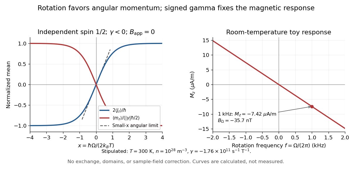
For a numerical example, stipulate $n=10^{28}{\mathrm{m}}^{-3}$, $T=300\mathrm{K}$, $\gamma =-1.76\times 10^{11}{\mathrm{s}}^{-1}{\mathrm{T}}^{-1}$, and rotation frequency $f=1000\mathrm{Hz}$. With $\Omega =2\pi f$, $\hslash =1.054571817\times 10^{-34}\mathrm{J}\mathrm{s}$, and $k_B=1.380649\times 10^{-23}J/K$, the model givesThese are teaching inputs and calculated outputs, not measured material values. The corresponding internal angular momentum density is $M_z/\gamma =+4.22\times 10^{-17}\mathrm{J}s/{\mathrm{m}}^3$. Keeping a rotor at prescribed $\Omega$ while its internal angular momentum changes requires the drive to supply the appropriate angular impulse. In an isolated body the mechanical part instead changes oppositely, as in magnetomechanical angular momentum balance. There is no creation of net angular momentum by choosing a rotating frame.

The two-state calculation is not a general formula for a ferromagnet. Exchange interactions, magnetic domains, magnetic domain-wall pinning, magnetic anisotropy, and hysteresis can determine which response is accessible. Both spin angular momentum and orbital angular momentum can contribute; a single constant gyromagnetic ratio may be only a restricted effective description. Rotation sets an internal bias, while the material and its preparation determine magnetization. The Barkhausen effect illustrates why a smooth bias can produce jumps instead of the toy smooth curve.

For a limited, reversible, isotropic linear model, suppose the same intrinsic volume magnetic susceptibility ${\chi }_v$ responds to the applied bias and to $B_{\Omega }/{\mu }_0$. For a uniformly magnetized ellipsoid along a principal axis, include its demagnetizing factor $N_d$:Solving this linear equation yieldsHere $H_{\mathrm{int}}$ and $H_{\mathrm{app}}$ are actual magnetic field intensities; the added rotational bias is an equivalent drive in the constitutive response. In SI, dimensionless ${\chi }_v$ multiplies an intensity in $A/m$, so $M_z={\chi }_v\Omega /\gamma$ would omit ${\mu }_0$ and have the wrong units. A susceptibility defined instead as $\partial M/\partial B$ has different units. State the convention before comparing formulas.

At zero applied magnetic field intensity, a stipulated ${\chi }_v=3$ gives prefactor $3/2$ in a sphere, with $N_d=1/3$, and a prefactor approaching $3$ in a long axial ellipsoid. This is a geometry check of the assumed linear model. A real cylinder does not have an exactly uniform demagnetizing field, and an irreversible ferromagnet cannot in general be represented by this single linear equation. Inferring an intrinsic gyromagnetic ratio requires an independently calibrated material response and a geometry-dependent conversion of the measured stray magnetic field.

The 2015 experiment used an air-driven nonmagnetic rotor containing polycrystalline gadolinium, with magnetic shielding and an external fluxgate magnetometer. Air drive reduced motor backgrounds. Measurements at 297–305 K were above the Curie temperature, at rotation frequencies up to 1.5 kHz. Reversing airflow reversed rotation and the magnetic signal; an empty capsule showed no speed-dependent signal. The readout measured stray magnetic field; geometry converted it to magnetization. Sample temperature was checked immediately after stopping. Heating and the conversion model limit inference.^[ref]

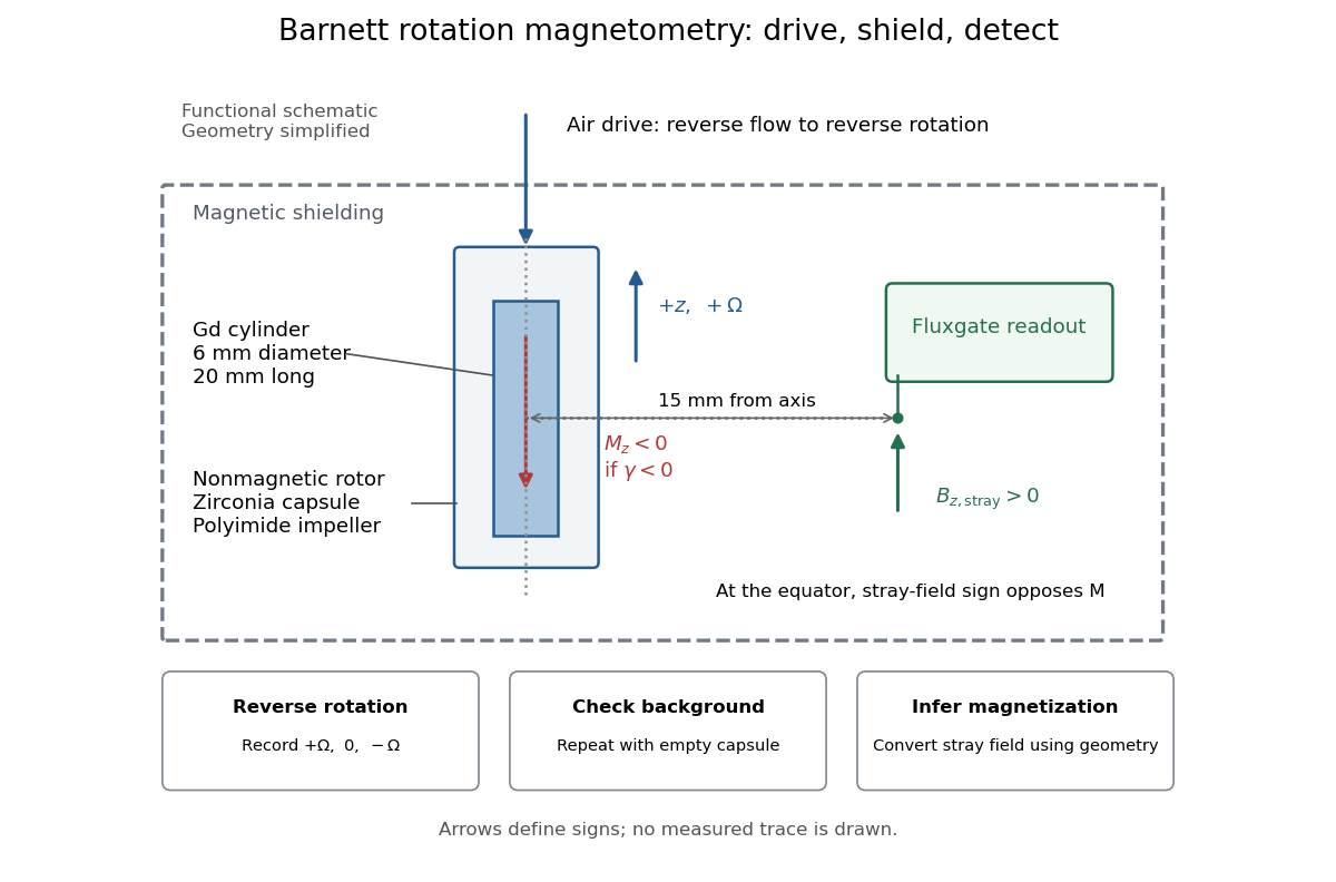
An additional analysis check follows from rotation symmetry. For signed sensor output $S$, separateAn ideal linear Barnett effect appears in the odd component; a fixed offset appears in the even component. This is a proposed diagnostic, not a claim about the paper's processing. A background correlated with direction can also be odd: reversal alone is insufficient. Empty-rotor checks, zero-speed readings, calibration of sensor polarity, and controlled temperature changes test different errors. Equatorial stray-field sign must also be converted to magnetization sign: for an axial magnetic dipole moment, the magnetic dipole field at its equator points opposite to that magnetic moment. The apparatus diagram makes this otherwise easy-to-miss sign change visible.