The Bohr model assumes circular electron orbits with quantized orbital angular momentum . It reproduces the hydrogen energy levels, but wavefunctions in quantum mechanics describe spatial probability distributions rather than definite trajectories. In particular, spherically symmetric Coulomb bound states have zero orbital angular momentum.
The puzzle is the coexistence of reproducible spectral lines and stable chemical atoms. A classical circular orbit in a Coulomb potential can have any negative energy: Coulomb's law alone selects no special radius or emitted frequency. Moreover, its electron has centripetal acceleration. The Larmor formula then predicts positive radiated power, so conservation of energy makes the orbit shrink. Simply drawing concentric circles explains neither stability nor a discrete spectrum.
Niels Bohr postulated nonradiating stationary states and emission with . His circular-orbit condition is . These assumptions override classical radiation; the emitted frequency need not equal an orbital frequency.[ref]
Consider a single electron of mass and a point atomic nucleus of mass and positive electric charge , with the elementary charge. Use nonrelativistic classical mechanics, omit external fields and interactions with other electrons, and writeHere is the Coulomb two-body reduced mass, the vacuum permittivity, and the Planck constant. The separation and relative speed describe the two-particle relative coordinate; neither body is silently pinned in place. The electron's own radius about the centre of mass is .
For the assumed circular orbit, Coulomb's law provides the required centripetal acceleration, and the imposed orbital angular momentum condition isSubstitute into the first equation and cancel to obtainThe kinetic energy is and the Coulomb potential energy is , with zero energy at infinite separation. HenceThis derives the energy sequence from the stated circular model; the modern Schrödinger equation derivation is the distinct series-termination quantization of the Coulomb radial equation. The radius above scales as , whereas the binding energy scales as . The Bohr radius article supplies the corresponding Coulomb potential length scale. The nonrelativistic assumption requires , with the speed of light.
For an original numerical example choose , , , , , , and . Treat these as stipulated constants for the calculation. They give , , and , where denotes an electronvolt. At , and ; the ground-state ionization energy is .
Taking gives . A finite nuclear mass reduces every binding energy by and increases each separation by . This follows from relative motion, not a fitted correction to individual spectral lines. Replacing the atomic nucleus by a heavier isotope changes the same factor, providing another check of the model.
For emission take integers . Applying conservation of energy to the model's internal energy difference, while neglecting the much smaller whole-atom photon recoil, givesThus Johannes Robert Rydberg's Rydberg formula is a difference of two energy levels expressed as a spectroscopic wavenumber. The same constants determine every line; there is no new parameter for each electronic transition. With the chosen inputs, . All wavelengths below are calculated in vacuum, not air, and are rounded model predictions rather than historical measurements.
The conventional names commemorate Theodore Lyman and Johann Jakob Balmer. Fixing produces the ultraviolet Lyman series, beginning with the Lyman-alpha line; fixing produces the Balmer series. As , the wavelength approaches : at the Lyman limit and for the Balmer series. Crowding follows directly from . Discreteness therefore coexists with a series limit.
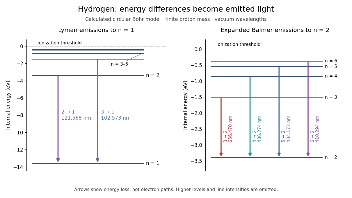
Correct line positions do not give wave intensities, lifetimes or electric-dipole selection rules for hydrogen. Those require a theory of the wavefunctions and their coupling to electromagnetic radiation. The circular model also omits spin, relativistic corrections and the Lamb shift. Its successful gross energy levels do not make its assumed orbits modern atomic orbitals.
In On the Constitution of Atoms and Molecules, Part I (1913), pp. 8–9, Niels Bohr interprets existing hydrogen discharge and astronomical spectra. Electrical discharge in a vacuum tube removes electrons; recombination supplies spectral lines. This is a theoretical interpretation, without a reported spectrograph of his own.[ref]
On the Constitution of Atoms and Molecules, Part I by Niels Bohr. Part I, section 2, pp. 8–9: existing spectra
An actual optical obstacle appears in Theodore Lyman's measurements: hydrogen discharge light entered an evacuated spectrograph directly through a slit, avoiding a transmitting window. A concave reflection diffraction grating dispersed the light onto photographic film. Pumping preserved the vacuum; a second slit supplied a known spectral displacement for wavelength calibration. Gas contamination and vacuum leaks limited the measurement. This apparatus resolved ultraviolet spectral lines; it did not image orbits.[ref]
Theodore Lyman, Pioneer of Ultraviolet Vacuum Spectroscopy by Paul Horowitz. Paul Horowitz, Theodore Lyman, Pioneer of Ultraviolet Vacuum Spectroscopy, pp. 3–4, figures 2–5: windowless discharge connection, grating, film, pumping and dual-slit calibration
For a separate original calibration exercise, suppose an idealized spectrograph returns synthetic vacuum line positions for , with chosen additive offset . Assume its dispersion scale is already known and only this offset is uncertain. Compare the finite-mass prediction with the fixed-nucleus prediction . Calibrate each model using only the line: . Then hold that offset fixed and test the other lines with residualsFor the finite-mass model every . The fixed-nucleus model has and residuals , , . Algebraically : one additive calibration cannot absorb a multiplicative change of the wavelengths. Allowing an unknown multiplicative dispersion factor as well would make the two models degenerate in this exercise, so independent scale calibration matters.
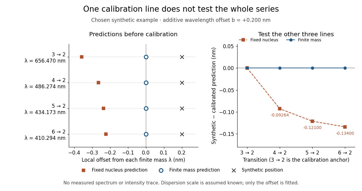
Balmer series predictions tested after calibrating one line
. Original synthetic calibration exercise with chosen . Left: finite-mass vacuum predictions and deliberately offset synthetic positions, displayed on a separate local wavelength axis for each line. Right: model residuals after anchoring the line; the remaining three lines test the prediction. Symbols are exact synthetic inputs and calculated results, not historical observations, error bars or an intensity trace. Details. Articles by others on the same topic

The Bohr model is a fundamental theory of atomic structure proposed by the Danish physicist Niels Bohr in 1913. It was developed to explain the behavior of electrons in atoms, particularly the hydrogen atom, and it marked a significant advancement in the field of quantum mechanics and atomic physics.



Was the first model to explain the Balmer series, notably linking atomic spectra to the Planck constant and therefore to other initial quantum mechanical observations.
This was one of the first major models that just said:
I give up, I can't tie this to classical physics in any way, let's just roll with it, OK?
It still treats electrons as little points spinning around the nucleus, but it makes the non-classical postulate that only certain angular momentums (and therefore energies) are allowed.
Bibliography:
- Inward Bound by Abraham Pais (1988) Chapter 9.e Atomic structure and spectral lines - Niels Bohr
- The Quantum Story by Jim Baggott (2011) Chapter 3 A Little Bit of Reality