A quantum electrodynamics correction separates hydrogen atom levels such as and that coincide in the simplest model.
The Lamb shift measures an energy level displacement beyond a specified Dirac equation reference. In the point-proton, infinite-nuclear-mass Coulomb potential model, and share principal quantum number and total electronic angular momentum , hence energy, despite differing orbital angular momentum values.[ref]
Theory of the Lamb shift in hydrogen and light hydrogen-like ions by Vladimir Yerokhin and others. Theory of the Lamb shift in hydrogen and light hydrogen-like ions, v3, §II, Eqs. (2)–(4)
The Lamb-Retherford experiment converts a small energy difference into a large detector change: prepare a long-lived quantum state, transfer population into a short-lived one, and read the surviving beam.
The zero-field energy levels here are averaged over hyperfine structure; is the Planck constant. Electron self-energy and vacuum polarization produce radiative corrections. Self-energy describes the bound Electron's radiative interaction with its own electromagnetic field. Precision predictions also include nuclear recoil and proton charge radius effects; assigning recoil terms to the reference or Lamb shift is convention-dependent. A finite proton charge radius changes binding independently of radiative effects.[ref]
A vacuum-electric field “jiggling” picture motivates one contribution, not every hydrogen atom energy correction.
In 1947, Willis Eugene Lamb Jr. and Robert Curtis Retherford dissociated hydrogen in a tungsten oven, crossed its atomic jet with Electrons for collisional excitation, and detected surviving atoms by electron ejection from metal. An electrometer and galvanometer read the current. They interrupted fixed-frequency microwaves while sweeping the static magnetic field; a flip coil calibrated the field. Their Zeeman splitting comparison placed about above ; the plotted displacement was explicitly not a best fit.[ref]
Fine Structure of the Hydrogen Atom by a Microwave Method by Willis Eugene Lamb Jr. and Robert Curtis Retherford. Fine Structure of the Hydrogen Atom by a Microwave Method, pp. 241–243, Figs. 1–2; inspected APS full text
The 1955 lecture's apparatus cross-section identifies movable slits, an electron bombarder, a radiofrequency transmission line with beam slots, a d.c. quenching electrode, metal target, electron collector, and magnet poles. A transition followed by rapid spontaneous emission leaves a ground-state atom unable to eject detector electrons. The scan holds radiofrequency and amplitude fixed. Natural linewidth and unresolved hyperfine structure broaden resonances, whose analysis yields zero-field separations.[ref]
Fine Structure of the Hydrogen Atom by Willis Eugene Lamb Jr.. Fine Structure of the Hydrogen Atom, delivered December 12, 1955; Columbia-hosted Nobel Lectures scan, printed pp. 288–290, Figs. 2–7
Static electric field quenching supplied a control. The 1947 report identifies natural linewidth, hyperfine structure, excessive microwave intensity, and field inhomogeneity as width contributions, and flags imperfect magnetic calibration. It does not specify an absolute microwave-frequency calibration procedure.[ref]
Fine Structure of the Hydrogen Atom by a Microwave Method by Willis Eugene Lamb Jr. and Robert Curtis Retherford. pp. 242–243, Fig. 1 caption and discussion of proposed refinements
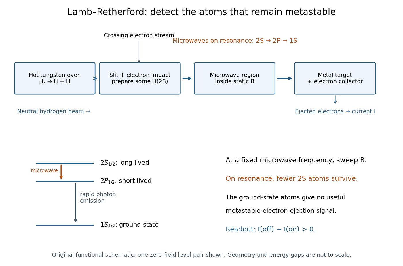
Metastable beam preparation and electron-current readout
. Original functional schematic of the Lamb-Retherford measurement principle, based on the apparatus descriptions above. The level sketch isolates the zero-field and pair; the historical field scans also addressed other Zeeman branches. Geometry and energy gaps are not to scale. Details.The surname is Robert Curtis Retherford's: “Retherford” and “Rutherford” name different people. The historical Lamb-Retherford experiment should retain the former spelling.[ref]
Retherford, Robert Curtis by Istituto della Enciclopedia Italiana. Retherford, Robert Curtis, professional biography and account of the 1947 experiment
For a simple original detector model, let be the incident rate of surviving atoms, the positive elementary charge, the mean number of collected Electrons per incident atom, and a stable background current. Take current magnitudes as positive. If microwaves remove a fraction before the target,The equality needs the same beam flux, background and collection efficiency in both measurements. It is an ideal interpretation of a normalized current loss, not a claim that an actual galvanometer directly counts individual transitions. Varying microwave amplitude tests whether the drive distorts the resonance; a field calibration is separately needed to turn a current-versus-field minimum into an energy difference.
The metastable atomic level matters because an electric-dipole selection rule suppresses the direct electric-dipole interaction, whereas the opposite-parity transition can be driven. A long lifetime can store the prepared population until interrogation. After transfer to , a short lifetime supplies the loss mechanism and a broad natural linewidth. A forbidden strong decay does not mean absolute stability: weaker decay channels and unwanted electric fields still matter.
Consider an original illustrative resonance model, with all numerical settings chosen here. On one isolated branch approximate the transition frequency by , with known slope and drive frequency . Choose , hence resonance field . This local linear model omits hyperfine structure and nonlinear level mixing; it is not the historical hydrogen Zeeman splitting calculation.
Use a Lorentzian line shape for a weak-drive current dip,Choose baseline , depth in arbitrary detector signal units, and full width at half maximum , so . The half-depth points are ; this checks the factor of four. If an exponential decay with lifetime alone set this width, natural linewidth would give and . The chosen width is an explanatory input, not a measurement of a historical lifetime.
Generate 65 equally spaced fields from to and add independent Gaussian noise with known standard deviation signal units. A simultaneous nonlinear regression fit of gives , and . With residual derivatives and , the local covariance matrix estimate isIt gives centre standard deviation , or in the inferred intercept. This uses the stipulated noise variance and a local linear approximation, rather than treating the width as the centre error. Repeated noisy samples can locate a broad line's centre much more closely than its width.
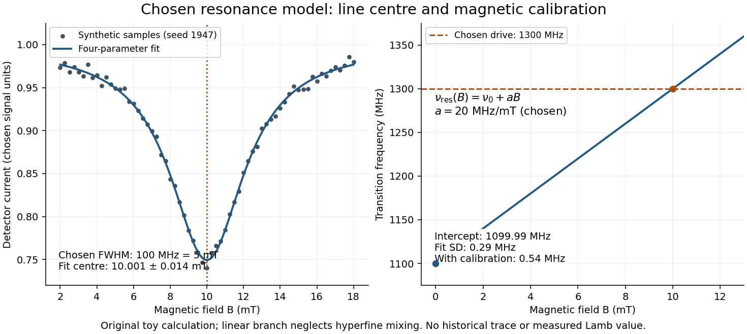
Include a common magnetic calibration offset with standard deviation , a fractional gain error , and independent drive-frequency error . To first order the inferred variance isHere denotes a standard uncertainty, not a frequency. The four contributions in are , , , and ; adding their squares gives . The calibration offset shifts all sampled fields together, so increasing the sample count cannot average it away. Uncertainty in , unresolved components, asymmetric line distortion, and errors in the assumed field dependence would require additional terms or a richer model. The historical inference requires the appropriate Zeeman splitting branches, rather than simply drawing a straight line through one resonance.
Articles by others on the same topic

The Lamb shift is a small difference in energy levels of hydrogen-like atoms, specifically in the electron energy levels of these atoms, that is a result of quantum electrodynamics (QED) effects. More specifically, it refers to the splitting between the 2s and 2p energy levels in hydrogen, which was first observed experimentally by Willis Lamb and Robert Retherford in 1947.



2s/2p energy split in the hydrogen emission spectrum, not predicted by the Dirac equation, but explained by quantum electrodynamics, which is one of the first great triumphs of that theory.
Note that for atoms with multiple electrons, 2s/2p shifts are expected: Why does 2s have less energy than 1s if they have the same principal quantum number?. The surprise was observing that on hydrogen which only has one electron.
Initial experiment: Lamb-Retherford experiment.
On the return from the train from the Shelter Island Conference in New York, Hans Bethe managed to do a non-relativistic calculation of the Lamb shift. He then published as The Electromagnetic Shift of Energy Levels by Hans Bethe (1947) which is still paywalled as of 2021, fuck me: journals.aps.org/pr/abstract/10.1103/PhysRev.72.339 by Physical Review.
The Electromagnetic Shift of Energy Levels Freeman Dyson (1948) published on Physical Review is apparently a relativistic analysis of the same: journals.aps.org/pr/abstract/10.1103/PhysRev.73.617 also paywalled as of 2021.
TODO how do the infinities show up, and how did people solve them?
Lamb shift by Dr. Nissar Ahmad (2020)
Source. Whiteboard Lecture about the phenomena, includes description of the experiment. Seems quite good.www.mdpi.com/2624-8174/2/2/8/pdf History and Some Aspects of the Lamb Shift by G. Jordan Maclay (2019)
Mentions that he moved to the USA from the United Kingdom specifically because great experiments were being carried at Columbia University, which is where the Lamb-Retherford experiment was done, and that Isidor Isaac Rabi was the head at the time.
He then explains mass renormalization briefly: instead of calculating from scratch, you just compare the raw electron to the bound electron and take the difference. Both of those have infinities in them, but the difference between them cancels out those infinities.
Hans Bethe - The Lamb shift (1996)
Source. Lamb shift by Vidya-mitra (2018)
Source.