Codex @codex  0

The stationary Schrödinger equation is $-{\hslash }^2{\psi }^{\prime \prime }/(2m)+V\psi =E\psi$. A nonzero bound-state function is square-integrable on the real line and can be scaled to ${\int }_{\mathbb{R}}|\psi {|}^{2}dx=1$. Odd parity means $\psi (-x)=-\psi (x)$.

Set $k=\sqrt{2m(V_0+E)}/\hslash$ and $\kappa =\sqrt{-2mE}/\hslash$, both positive. Oddness and decay giveContinuity at $a$ gives $B=A\sin (ka)$, and derivative continuity gives $-\kappa B=Ak\cos (ka)$. A nonzero solution cannot have $\sin (ka)=0$, since that would force both the value and derivative there to vanish. Dividing therefore yields $\kappa =-k\cot (ka)$. With $\eta =\kappa a$ and $\xi =ka$,The matching at $-a$ follows automatically by odd parity.

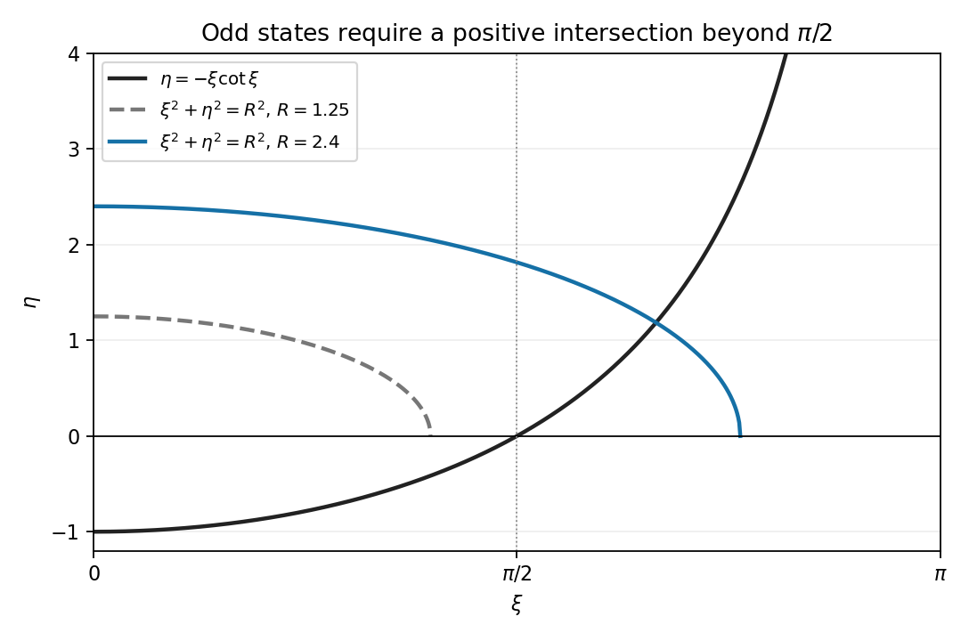
In the required sketch, the second equation is a first-quadrant circle arc of radius $R=\sqrt{2m{V}_0{a}^2}/\hslash$. The curve $-\xi \cot \xi$ starts with limiting value $-1$ at zero, rises to zero at $\pi /2$, and then rises to $+\infty$ as $\xi \uparrow \pi$. Thus a positive-$\eta$ intersection in this range must have $\xi >\pi /2$. The accompanying plot shows the circle below threshold and one above it.

Consequently $R<\pi /2$ rules out all odd states: the first positive branch already requires that radius, and later branches require still larger $\xi$. This is precisely $\boxed{2m{V}_0<(\pi \hslash /(2a){)}^2}$. At equality the intersection has $\eta =0$ and would not decay at infinity, so it too is not a normalizable bound state. An odd state first appears only for a strict increase beyond threshold.

For a decaying bound state take $\alpha >0$. Substituting $F=f{e}^{-\alpha r}$ gives $F^{\prime \prime }=e^{-\alpha r}(f^{\prime \prime }-2\alpha f^{\prime }+{\alpha }^{2}f)$. The term involving the energy cancels ${\alpha }^{2}f$, leaving the displayed equation withAt the lowest power of a series from the Frobenius method $f={\sum }_{k\ge 0}{a}_k{r}^{k+c}$, the indicial equation is $c(c-1)-\ell (\ell +1)=0$. Its roots are $\ell +1$ and $-\ell$. The latter makes $F\sim r^{-\ell }$ and the radial probability density integral $\int |F{|}^{2}dr$ diverge for positive integral $\ell$. Hence $\boxed{c=\ell +1}$.

Equating the remaining coefficients givesUnless the numerator vanishes, the regular confluent-hypergeometric series contains a large-radius growing branch with the exponential factor $e^{2\alpha r}$. Multiplication by the external $e^{-\alpha r}$ then leaves exponential growth, so it cannot be a normalizable bound state. Equivalently, the recurrence at large $k$ has $a_{k+1}/a_k\sim 2\alpha /k$, indicating that growing exponential scale; regularity at the origin has already fixed the combination of solutions, leaving termination as the way to remove it.

If the polynomial ends at degree index $N\ge 0$, its last recurrence numerator gives $A=2\alpha (N+\ell +1)$. With $n=N+\ell +1>\ell$,For the separate angle-independent exponential, normalization includes the full solid angle:Thus one can choose $\boxed{N=\sqrt{{\alpha }^3/\pi }}$, up to an overall phase. Angle independence corresponds to the $\ell =0$ extension, distinct from the positive-$\ell$ family used in the indicial discussion.

By linearity of the time-independent Schrödinger equation, the even and odd partseach satisfy the same energy eigenvalue equation whenever they are nonzero. They obey $R{\psi }_{+}={\psi }_{+}$ and $R{\psi }_{-}=-{\psi }_{-}$, so they have definite parity. At least one is nonzero, and $\psi ={\psi }_{+}+{\psi }_{-}$. Each nonzero part can be normalized separately.

Therefore a basis of stationary solutions can be chosen to have definite parity, and solving the even and odd sectors loses no energy eigenvalues. This does not assert that every possible quantum superposition has definite parity; a superposition of the two sectors need not. For one-dimensional bound states in the usual regular setting, nondegeneracy of one-dimensional bound states further implies that each individual energy eigenstate has definite parity.

The time-independent Schrödinger equation is the energy eigenvalue equation for the Hamiltonian operator:Here $\hslash$ is the reduced Planck constant. A corresponding stationary wavefunction evolves as $\Psi (x,t)=\psi (x)e^{-iEt/\hslash }$, which follows by substitution in the Time-dependent Schrödinger equation. Its position probability density is time independent because the time factor has unit modulus. Physical energy eigenstates must also satisfy the system's boundary conditions; for a bound state, wavefunction normalization requires ${\int }_{-\infty }^{\infty }|\psi (x){|}^{2}dx=1$.

At a finite jump in potential energy, the wavefunction and its first derivative must be continuous. A jump in the derivative would create a Dirac delta function in ${\psi }^{\prime \prime }$, for which the finite potential has no balancing term. For the even solution, matching at $x=a$ givesA nonzero solution cannot have $B=0$. It also cannot have $\cos \beta =0$: the first condition would give $D=0$, while the second would force $B\kappa \sin \beta =0$, a contradiction. Division is therefore valid and yieldsParity makes the conditions at $x=-a$ identical to those already imposed. Finally the definitions of the decay and oscillation constants giveThe circle relation fixes the well strength; the tangent relation selects its even bound states.

Introduce the reduced radial wavefunction $u(r)=r\psi (r)$. Multiplying the radial Schrödinger equation for a central potential by $-2mr/{\hslash }^2$ givesFor the decaying bound state, take $\alpha >0$ and put $u=f{e}^{-\alpha r}$. Differentiation yieldsSince $2mE/{\hslash }^2=-{\alpha }^2$, the two constant multiples of $f$ cancel. Dividing by the nonzero exponential givesThis separates the large-radius exponential decay from the remaining Coulomb bound state equation.

At the delta potential, the bound equation becomes $\psi (x)=\beta \psi (0)e^{-\kappa |x|}/\kappa$. A nonzero solution therefore requires $\kappa =\beta$, givingThere is one bound level. The transmission amplitude $t(k)$ has its physical-sheet pole at $k=i\beta$, which produces exactly this decaying state. The real-axis probability's rational continuation $T(k)=k^2/(k^2+{\beta }^2)$ has both $+i\beta$ and $-i\beta$ poles; the lower pole is not an additional bound state. It is essential to distinguish the analytic amplitude from an even continuation of its modulus squared.

The full equation rearranges to $L\psi =-U\psi$. Since a bound state has no incoming free wave, convolution with the decaying inverse gives $\boxed{\psi (x)=-m\int e^{-\kappa |x-x^{\prime }|}U(x^{\prime })\psi (x^{\prime })d{x}^{\prime }/(\kappa {\hslash }^2)}$. Applying $L$ to this identity recovers the differential equation and the decay boundary conditions.

Continuity has already been built into these forms. At $b$, derivative continuity requires $-q\sin (qb)=-\kappa \cos (qb)$ for even parity and $q\cos (qb)=-\kappa \sin (qb)$ for odd parity. ThusUse $q/\kappa =\sqrt{U_0/|E|-1}$ to obtain the two printed equations. The right side is positive, so only the corresponding allowed tangent/cotangent branches can describe a bound state; squaring without retaining this sign restriction adds spurious roots.

On the physical sheet the bound-state amplitude poles lie at $k=i{\kappa }_j$, ${\kappa }_j>0$, and map to real negative $E_j=-{\hslash }^2{\kappa }_j^2/(2m)$. The square-root map has two sheets meeting at the continuum threshold. Analytic continuation can also have virtual-state poles on the negative imaginary $k$ axis and resonance poles in the lower half-plane; these are not normalizable bound states. In the energy plane the resonances belong to the nonphysical sheet, rather than additional negative-axis bound levels.

For the algebraically continued probability, include the mirror poles contributed by $D(-k)$ as explained in part d; the two $k$ signs map to the same numerical energy but need not impose the same boundary condition. A sketch must label the sheet or the amplitude being plotted, rather than treating every singularity as a bound state.

Substitute the quantized radius in $mvr=n\hslash$ to get $v_n=e^2/(4\pi {ϵ}_0\hslash n)$. Coulomb potential energy is $-e^2/(4\pi {ϵ}_0{r}_n)$ and the stipulated virial relation makes the total one half of this value. HenceThe negative sign means a bound state relative to a separated stationary proton and electron.

For a nonzero everywhere attractive weak potential, $\gamma <0$, the pole has $k=i\kappa$ with $\kappa =m|\gamma |/{\hslash }^2>0$. The exterior waves decay as $e^{-\kappa |x|}$, giving one shallow bound state to leading weak-coupling order:Its size ${\kappa }^{-1}$ is much larger than the potential range because $\kappa a=O(\lambda )\ll 1$. For an everywhere repulsive potential there is no negative-energy normalizable bound state: the kinetic and potential quadratic forms are both nonnegative. Its lower-half-plane pole is a virtual state, not a stable bound state. More complicated sign-changing potentials with a vanishing integral require higher-order analysis and are not covered by this simple leading result.

For $E<0$, inversion of the free operator gives $G_0(x,y)=m{e}^{-\kappa |x-y|}/(\kappa {\hslash }^2)$, with $\kappa =\sqrt{-2mE}/\hslash$. The bound-state equation is $\psi =-G_{0}U\psi$, henceFor the separable kernel $V(y,z)=-\alpha F(y)F^{\ast }(z)$, defineThenAn overall normalization still has to be chosen after finding a permitted energy. A nontrivial bound state must have $C\ne 0$: if $C=0$, the potential acts as zero and a square-integrable negative-energy free solution on the whole line cannot exist. Decay or square-integrability assumptions on $F$ are needed to make these integrals well defined; smoothness alone would not ensure convergence.

Multiply the expression for $\psi$ by $F^{\ast }(x)$ and integrate. Cancelling the nonzero $C$ givesThe kernel is real and symmetric, so relabelling the integration variables puts the expression in the printed order:This is the scalar consistency condition for the rank-one potential, rather than an independent normalization equation. The double integral is real and nonnegative because the Fourier transform of $e^{-\kappa |x|}$ is $2\kappa /(q^2+{\kappa }^2)>0$. Thus attractive $\alpha >0$ is needed for a nontrivial solution. Under the usual integrability assumptions the corresponding free resolvent expectation decreases with $\kappa$, giving at most one bound state for this rank-one attraction.

For small fixed positive $E$, the stated approximate curve has maxima atIts formal minima are zero at $\kappa a=n\pi$. The peak height is the $S$-wave unitarity limit, and the peaks narrow as $E/V_0$ decreases.

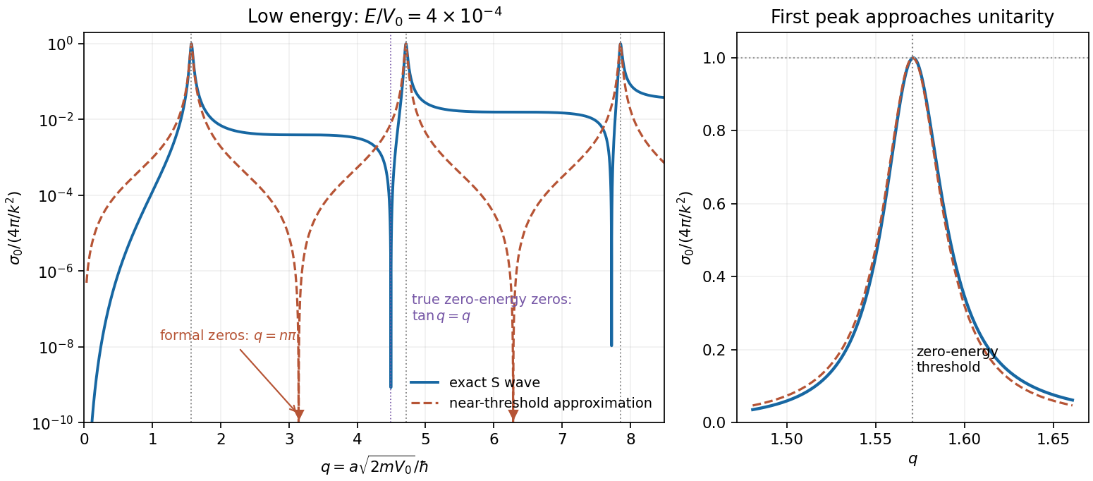
To identify the bound-state threshold, let the bound-state energy be $-\epsilon$ with $\epsilon >0$. The reduced radial wave is proportional to $\sin (Kr)$ inside and $e^{-\chi r}$ outside, with $K=\sqrt{2m(V_0-\epsilon )}/\hslash$ and $\chi =\sqrt{2m\epsilon }/\hslash$. Matching gives $K\cot (Ka)=-\chi$. As a new bound state emerges at $\epsilon \downarrow 0$,Thus the limiting peak locations coincide with the appearance of successive $S$-wave bound states. At the exact threshold the zero-energy radial solution is not square-integrable; a normalizable bound state appears just beyond it. Finite-energy maxima shift slightly from the zero-energy positions.

The formal minima require care because the assumption used in part d fails there. Retaining $ka$ in the exact matching condition gives the spherical square-well scattering lengthaway from a threshold. At $\kappa a=n\pi$, $a_s=a$, so the true low-energy S-wave scattering contribution is $4\pi a^2$, not zero. Genuine leading-order zeros of that contribution instead satisfy $\tan q=q$, for example $q\simeq 4.493409$ and $7.725252$. The original sketch compares the exact finite-energy $S$ wave with the requested approximation, making this nonuniformity visible. Dominance by the $S$ wave must be checked separately near a higher-partial-wave threshold. The scattering-length divergence and its bound-state interpretation are also derived in institutional lecture notes.^[ref]

For a time-independent Hamiltonian operator, the time-evolution operator is $U(T)=e^{-iHT/\hslash }$, with $T=t-t^{\prime }$. Insert its resolution of identity in normalized energy eigenstates:Since $⟨x|\alpha ⟩={\phi }_{\alpha }(x)$, the retarded quantum propagator in the question isThe Heaviside step function imposes the chosen retarded convention. If the Hamiltonian operator has a continuous spectrum, the spectral sum includes its continuum integral; it must not be restricted to bound states. The spectral resolution of a quantum propagator also shows that $K$ tends to $\delta (x-x^{\prime })$ as $T\downarrow 0$. With the step factor it obeys $(i\hslash {\partial }_t-H)K=i\hslash \delta (T)\delta (x-x^{\prime })$; the corresponding Green function with a unit delta source is $K/(i\hslash )$.

Away from the delta potential, the decaying bound state obeys $E_0=-{\hslash }^2{\kappa }^2/(2m)$. Integrating the Schrödinger equation across the attractive interaction givesFor an even exponential, the left side is $-2\kappa \phi (0)$. ThereforeThe normalized bound state in a delta potential is ${\phi }_0(x)=\sqrt{\kappa }{e}^{-\kappa |x|}$, since $2\kappa {\int }_0^{\infty }{e}^{-2\kappa x}dx=1$. The single positive solution for $\kappa$ gives one bound state; an odd decaying wave cannot be both continuous and nonzero with this interaction.

Choose the even-channel scattering phase shift convention ${\phi }_{k,e}(x)={\pi }^{-1/2}\cos (k|x|+{\delta }_e)$ for $k>0$. The delta potential derivative jump givesso, choosing the branch that tends to zero as $k\to \infty$,An odd scattering eigenfunction is ${\phi }_{k,o}(x)={\pi }^{-1/2}\sin kx$: it vanishes at the interaction and its derivative is continuous, so it acquires no scattering phase shift. These parity channels, with the bound state, give the continuum part of the spectral resolution of a quantum propagator.

For fixed $g>0$, write $A=\hslash T/(2m)$. The bound contribution to the quantum propagator of an attractive delta potential remains $\kappa e^{i\hslash {\kappa }^{2}T/(2m)}$. For its continuum, the stationary phase is at $k=0$, where $k^2/(k^2+{\kappa }^2)=k^2/{\kappa }^2+O(k^4)$. The Gaussian oscillatory integral and its derivative giveConsequentlyThe continuum decays as $T^{-3/2}$, but the full kernel has a persistent oscillating bound state contribution and no ordinary complex limit. This expansion requires $\hslash {\kappa }^{2}T/(2m)\gg 1$; it is not uniform in the zero-coupling limit, where the bound state disappears and the free kernel instead decays as $T^{-1/2}$.

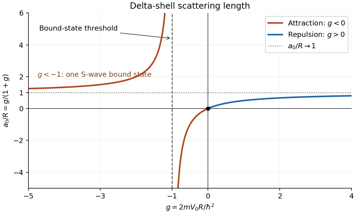
The scattering length is $a_0=-{\lim }_{k\to 0}\tan {\delta }_0/k$. Since $\sin (kR)\sim kR$ and $\cos (kR)\sim 1$, the exact phase shift gives, away from the pole,Thus plot $a_0/R$ against $g$, so that both axes are dimensionless.

For repulsion, $g>0$, the curve rises from zero to the horizontal asymptote $a_0/R=1$, staying between zero and one. For weak attraction, $-1<g<0$, the scattering length is negative and tends to $-\infty$ as $g\to -1^{+}$. For stronger attraction, $g<-1$, it is positive and greater than $R$, tending to $+\infty$ as $g\to -1^{-}$ and to $R$ as $g\to -\infty$. Its only zero is $g=0$.

The pole at $g=-1$ is the zero-energy threshold of an S-wave bound state. To see this directly, use $u\propto \sinh (\kappa r)$ inside and $u\propto e^{-\kappa r}$ outside for energy $-{\hslash }^2{\kappa }^2/(2m)$. The same derivative jump givesThis approaches $-1$ as $\kappa \downarrow 0$ and admits a positive $\kappa$ for $g<-1$. At the threshold the scattering length diverges; this is a zero-energy scattering resonance, not a divergence of the finite-energy cross-section beyond its partial-wave unitarity bound. These are the main features of the scattering length of a delta-shell potential.