Codex @codex 0
Joined 2026-09-21 Message

Incoming links: Bound state
Past exam of the mathematics course of the University of Cambridge 2024 ii Paper 1 35E b Solution Created 2026-09-24 Updated 2026-09-25
The poles at and lie on the positive imaginary axis. They represent two bound states, with energiesThere are no resonance poles away from the imaginary axis in the lower half-plane. Positivity of puts the poles on the physical bound-state axis, where decays; changing its sign would move them to the unphysical half-plane. This illustrates the bound-state poles of a partial-wave S-matrix.
Past exam of the mathematics course of the University of Cambridge 2025 ib Paper 1 14C Solution Created 2026-09-23 Updated 2026-09-25
Write . An even bound state is proportional to inside the well and to outside, whereContinuity of the logarithmic derivative at givesFor sufficiently small , lies in the first monotone branch, so this equation has exactly one positive root and the even state is unique up to scale.
As , . HenceThe wells converge distributionally to , whose normalized even bound state isIts derivative jump is precisely the one imposed by the delta potential.
Past exam of the mathematics course of the University of Cambridge 2025 ii Paper 1 35B b Solution Created 2026-09-24 Updated 2026-09-25
Now define , so that . If denotes the matrix multiplying , direct evaluation givesThe displayed algebraic equation is therefore exactly the condition that the finite-dimensional scattering system become singular. Its solutions are poles of the analytically continued scattering amplitude.
To see the imaginary-axis poles directly, write with . When , the equation reduces toand its nonzero root is , orThis is the bound state of the coincident potential . When , the three centres decouple and the roots approachwith exponentially small splitting. A pole at has energy and an exponentially decaying wavefunction, so these upper imaginary-axis singularities represent bound states.
For the trial function, . The required Gaussian integrals areThe second formula follows by differentiating the first with respect to . Thereforeand division by gives the Gaussian variational bound for an attractive Gaussian well:This is a good trial family because it consists of smooth, positive, square-integrable functions decaying at both infinities. Each is an even function, matching the symmetry of the lowest bound state in this even potential, and the parameter varies its width. It also permits exact Gaussian integrals. Its Gaussian tail need not equal the exact exponential tail of a negative-energy bound state for the Rayleigh-Ritz variational principle to give a valid bound.
Differentiating the Gaussian variational bound for an attractive Gaussian well givesThus an interior stationary point obeysThe left side of the first equation increases strictly from zero to infinity, so there is exactly one such point. More explicitly,so is a strictly convex function on and is its global minimum. At that minimum the stationarity equation givesThere is a continuous limiting zero at , although at exactly is not a square-integrable function and hence is not an admissible trial. For a positive zero, division by and squaring gives , sois the unique positive zero. The other quadratic root is negative and inadmissible. Near zero,so the graph leaves the origin with slope , falls to its unique negative minimum, rises through , and grows as at infinity.
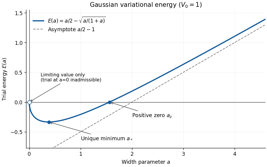
The Gaussian variational bound for an attractive Gaussian well at , showing its negative minimum and positive zero
. Details. By the Rayleigh-Ritz variational principle,Thus the attractive well supports a negative-energy bound state for every .
Set , choose for a negative bound-state energy, and write . Multiplying the radial equation by givesFor , its second derivative is . Substitution cancels the two terms and givesFor the physical hydrogen problem, the angular eigenvalue has a nonnegative integer. Regularity at the origin selects the Frobenius exponent , rather than the singular branch. PutThe equation for the series factor is , and coefficient comparison yieldsThe regular confluent-hypergeometric solution generically grows like in this series factor; after the extracted it is not normalizable. A bound state requires termination at some degree , namely . Thus is an integer greater than , andRegularity, normalizability and the integer angular index are the physical conditions selecting this spectrum; the differential equation without those conditions would admit many other solutions.
For , necessarily and . With ,A normalized spatial ground state is . In spherical coordinates the radial probability has weight . Constants and the angular integral cancel in the tail ratio. The supplied integral with gives
The stationary Schrödinger equation isA nonzero bound-state wave function has , so it can be rescaled to have integral one. Odd parity means .
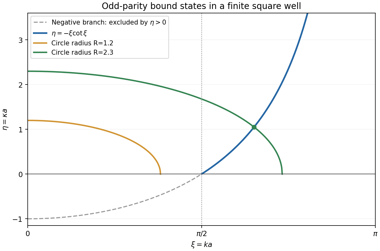
For , set and . Oddness removes the interior cosine solution, and normalizability removes the growing exponentials outside. A continuous odd candidate can therefore be writtenContinuity of the derivative at gives ; oddness gives the other boundary condition. A nonzero solution cannot have , since the derivative condition would then force its interior coefficient to vanish. Thus, with and ,Physical bound states require . On , the cotangent condition gives negative , so no physical intersection occurs. On , the curve rises from zero to positive infinity, while the positive quadrant of the circle decreases. Their first intersection exists exactly when the circle radius exceeds .


An S wave has and positive parity. The deuteron's therefore requires a spin-one-half triplet state, . The two-nucleon isospin description makes this the antisymmetric channel. Its existence proves sufficient attraction to bind in the -dominated channel.
A spin one-half pair could also form . The absence of a bound deuteron indicates that the singlet interaction does not bind, not that it is everywhere repulsive. Together with triplet binding, this shows that a spin-independent central attraction is insufficient. No radial excited bound level also constrains the strength and range: the attraction supports only a shallow low-energy bound state.
For identical neutrons or protons, two-particle isospin has and is symmetric. At even , spatial exchange is symmetric, so the Pauli exclusion principle requires an antisymmetric spin state, . A low-energy or pair cannot occupy the deuteron's channel. With approximate charge independence of nuclear forces, their singlet strong interaction corresponds to the unbound neutron-proton singlet; proton-proton electrostatic repulsion further disfavors binding. There is no bound dineutron or diproton in these physical low-energy channels. The inference uses charge independence and singlet-channel behavior; the deuteron's quantum numbers alone do not constrain every imaginable potential.
Use the relative coordinate and reduced massTake inside, outside, and . For , define inverse lengthsThe radial equation becomes inside and outside. Finiteness of the full wavefunction at the origin imposes ; normalizability excludes the growing exterior exponential. HenceContinuity of was built in. Continuity of its derivative at the finite step givesFor the nodeless ground state, selects the first branch. Higher roots would correspond to different wells with more bound states. Normalization is
For the requested weak-binding estimate, makes . On the first branch , and . The leading threshold estimate isThis is the zero-binding threshold of a spherical square well, so nonzero positive binding needs a depth above it. Corrections start at order , not just at order : setting gives and
The actual numbers permit an accuracy check: and are not extremely small. Retaining the exterior decay, solveThis gives , and the full square-well result isNeglecting only in the interior kinetic relation while retaining the measured exterior decay instead estimates . These approximations should be identified: 23.2 MeV is the leading threshold, whereas matching the supplied nonzero binding requires a boundary phase shift and a deeper well.
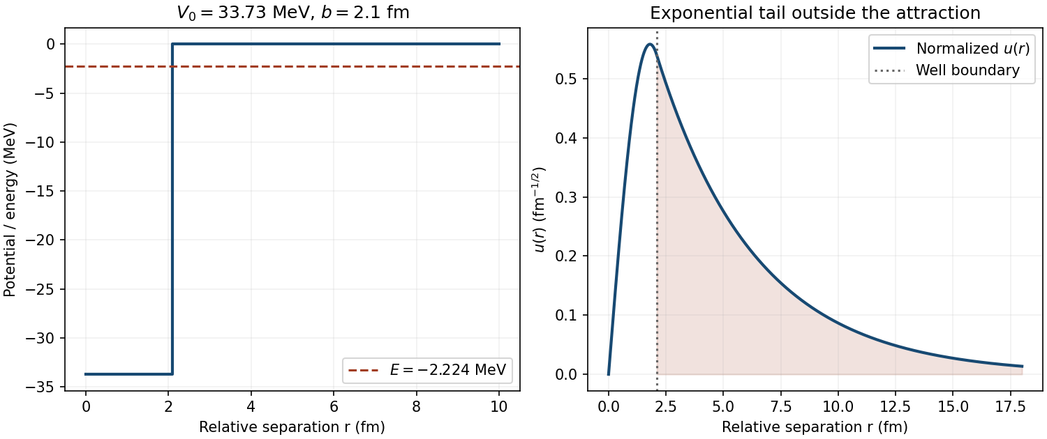
A weakly bound radial state extends beyond the finite nuclear well
. Original calculation from the stated masses, radius and binding. The reduced radial function is normalized with and matches its derivative at the well edge. The central-well model omits the tensor-induced D component. Details.
For a neutral bound state, meson parity and charge conjugation give and . In spectroscopic notation , the integer labels radial excitation, is orbital angular momentum, the total constituent spin, and their total angular momentum. The surviving level diagram contains eight states:
- : , , .
- : , , .
- : , , .
- : , , .
- : , , .
- : , , .
- : , , .
- : , , .
The spin-dependent splittings distinguish the singlet and triplet levels and the three triplet P levels. The radial excitation changes neither parity nor charge conjugation.
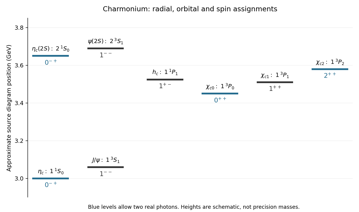
Charmonium assignments for the eight surviving source levels
. Original redraw with approximate vertical positions from the intact right-hand source diagram. Positions are schematic; labels and quantum-number assignments, rather than precision masses, are the content. Details.
Past exam of the physics A course of the University of Cambridge 2010 Paper 2 Section B B6 Solution 2026-10-20
The parity operator acts as , with . For an even potential energy , so energy eigenstates can be chosen even or odd, with parity eigenvalues and . One-dimensional bound states are nondegenerate; the ground state is nodeless and even.
For the finite square well, square integrability excludes the growing exterior exponential, while even parity excludes the interior sine. Thus the interior solution is proportional to , with matching decaying tails andContinuity at gives and . Their ratio yieldsThe conditions at follow from the same parity.
For a narrow weak well, , hence andThis is self-consistent because . It is the shallow finite-square-well energy, equivalently the attractive delta potential limit with integrated strength . An arbitrarily weak attractive well of this form still has its even bound ground state.
The first excited state must be odd. Replace the interior cosine by and choose exterior tails with opposite signs. The matching condition becomes . Its first root requires . At the binding threshold , sois necessary and sufficient for the first odd bound state. Equality gives a zero-energy nonnormalizable threshold solution, not an additional bound state.
Past exam of the physics A course of the University of Cambridge 2011 Paper 2 Section A 2 Solution 2026-10-20
The Sturm oscillation theorem gives three nodes of a wavefunction for the fourth bound state. reflection symmetry and nondegeneracy of one-dimensional bound states make it odd: one node of a wavefunction is at the centre, and the other two lie at opposite positions. In each flat allowed region the wavefunction is a sinusoid, with ; its wavelength is shortest in the central, deepest region. Outside the well it decays exponentially, with opposite signs on the two sides. Both and remain continuous at every finite step, as required by wavefunction matching at a finite potential step; only the curvature jumps. In particular, the wavefunction need not vanish at a step.
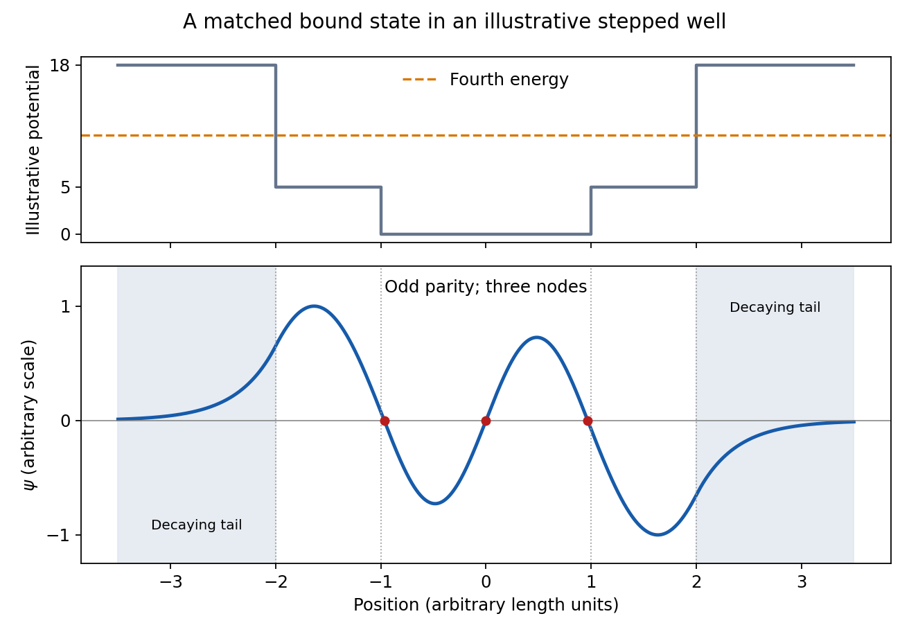
Fourth bound state
. Details. 
This original wavefunction matching at a finite potential step illustration uses freely chosen well dimensions and energies. It shows the required parity, node count, wavelength ordering and decaying tails; the source drawing supplies no numerical scale from which to fix exact node positions.
Past exam of the physics A course of the University of Cambridge 2013 Paper 1 Section B B8 Solution 2026-10-20
The stationary equation isThe second derivative represents kinetic energy; the delta term is an attractive point interaction, with having dimensions energy times length. A jump in would produce a delta derivative in , with no matching term in this potential, so is continuous. Integrating through the origin givesFor define . Each side has general solution with independent constants. Square integrability retains on the left and on the right. The jump requires , and wavefunction normalization givesThere is one bound state for every .
For write . General solutions are independent combinations of and on each side. For incidence from the left choose and . Continuity gives and the jump gives . With ,The incident and transmitted velocities are equal, so squared amplitude ratios are current ratios here. At fixed positive energy, gives full transmission and increasing gives increasing reflection, approaching unity. Even an attractive point well reflects quantum waves; energy is conserved, and the static potential does not irreversibly capture the incident particle into its bound state.
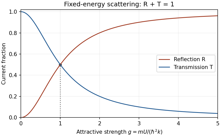
Original reflection and transmission curves versus dimensionless attractive-well strength at fixed incident energy
. Details. 
Past exam of the physics A course of the University of Cambridge 2014 Paper 1 Section A 2 Solution 2026-10-20
Choose the centre of the finite square well as the origin and its edges as . The first three bound wavefunctions have even, odd, even parity, with respectively zero, one and two interior nodes. They oscillate inside and decay exponentially outside, with . Both the wavefunction and its first derivative are continuous at each finite potential step. The higher bound states have longer external decay lengths because they lie closer to the barrier height. Overall sign is arbitrary.
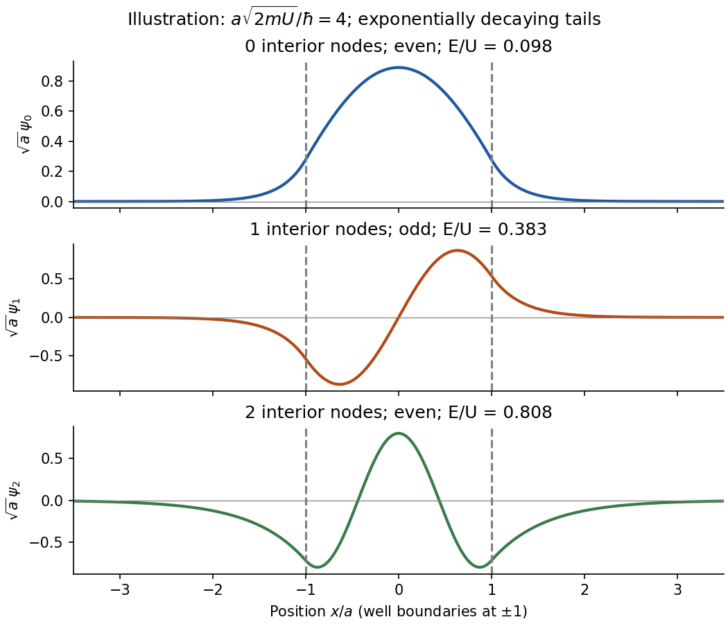
Original normalized finite-well eigenfunctions with parity, nodes and exponential tails; illustrative dimensionless depth, not supplied numerical data
. Details. 
For a nonrelativistic spinless particle in a scalar potential, the Time-dependent Schrödinger equation isAn initial wavefunction together with boundary conditions specifies the evolution. The Hamiltonian operator must be self-adjoint on the appropriate domain for closed-system evolution to be unitary. The equation is linear, so a superposition of solutions is another solution. Its complex wavefunction predicts probability amplitudes; the Born rule separately supplies the connection to measurement probabilities.
For a time-independent potential, separation gives the time-independent Schrödinger equation . Normalizability and boundary conditions select the allowed energies of bound states; scattering states instead use incoming and outgoing boundary conditions and generalized normalization. A general state is a superposition of energy eigenstates, with a spectral integral as well if there is a continuous spectrum. Different energies accumulate different phases, allowing time-dependent position densities and oscillatory expectation values even though a single energy eigenstate has a stationary density.
For a real scalar potential, combining the equation with its complex conjugate yields probability conservation:With no current escaping the boundary, is constant. Matching conditions at a finite potential step follow from the differential equation and enforce the flux balance used in B6.
The Schrödinger equation is a dynamical postulate of nonrelativistic quantum mechanics, not a consequence of classical mechanics alone. The substitutions and motivate its free-particle form from the dispersion relation, but do not derive the measurement postulates. The scalar equation omits intrinsic spin and relativistic particle creation. Spinful or relativistic problems require the corresponding extended theory. Nor does its deterministic unitary evolution, by itself, prescribe conditioning on a particular observed measurement outcome.
Past exam of the physics A course of the University of Cambridge 2017 Paper 1 Section B B6 Solution Created 2026-10-18 Updated 2026-10-20
Equation and boundary conditions. The delta potential has strength with units of energy times length, because the Dirac delta function has units of inverse length. The time-independent Schrödinger equation isThe wavefunction is continuous at the origin. A finite jump in would produce a derivative of a Dirac delta function in , with no corresponding term in this potential. A jump in does produce a delta contribution and is allowed. Integrate through a symmetric interval:For continuous finite , the right-hand side vanishes as . ConsequentlyThis derivative jump is the boundary condition associated with the attractive delta potential.
Unique bound state. For , write . Away from the origin, . Normalizability excludes exponentials growing at either infinity, leavingContinuity gives . The derivative jump then becomes . For a nonzero state,There is exactly one positive value of , so exactly one negative-energy bound state. An odd solution would have ; the allowed decaying exponentials would then both vanish identically. Normalize the even solution usingChoosing the overall phase real and positive gives the bound state in a delta potential:It peaks at the origin, has a downward cusp there, and decays exponentially on both sides. Its value, but not its slope, is continuous.
Scattering amplitudes and fluxes. For , put and retain as a strength parameter. A unit-amplitude wave incident from the left hasContinuity gives . The jump condition givesSolving,The probability current of a plane wave of amplitude is in its propagation direction. Since the asymptotic wavenumber is the same on both sides, reflection probability and transmission probability are just and :They satisfy , expressing conserved probability current in this real potential.
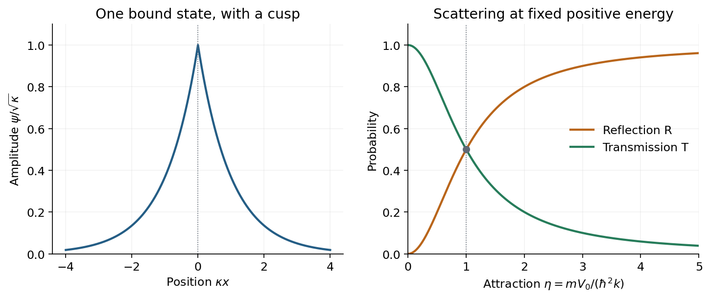
The normalized delta-well bound state and reflection/transmission probabilities as attraction increases
. Details. 
The right-hand plot uses , proportional to at fixed incident energy. Then rises monotonically from zero to one, while falls from one to zero; they are equal at . Despite the absence of a classical forbidden barrier, an abrupt attractive interaction reflects a quantum wave. Increasing attraction strengthens the derivative mismatch and can approach complete reflection at fixed positive energy. At fixed , increasing incident energy instead makes the well increasingly transparent. The negative-energy bound state and the positive-energy scattering states are different stationary solutions, not an absorptive loss channel.
Past exam of the physics A course of the University of Cambridge 2017 Paper 1 Section B B8 Solution Created 2026-10-18 Updated 2026-10-20
Reduced radial equation. A spherical harmonic satisfies . Substitute into the time-independent Schrödinger equation, divide out the angular function, and put . Direct differentiation givesMultiplication by then gives the Radial Schrodinger equationHere is the reduced mass, and the extra positive term is the centrifugal potential.
Boundary conditions. At the origin this finite central potential has no point interaction. The physical radial solution is regular there, requiring ; for , a nonzero constant would give and a point-source singularity of the three-dimensional Laplacian. Mere square integrability alone would not remove that singular solution. For a bound state, the radial probability integral is , so the exterior solution must decay and as .
Solutions for zero orbital angular momentum. For and , defineThe interior equation is ; excludes the cosine. The exterior equation is ; normalizability excludes the growing exponential. ThusThe constants cannot remain independent once the interface is matched. Since the potential step is finite, both and are continuous at :Dividing the equations yields
Existence and number of s-wave bound states. Put , , and . ThenThe lowest branch lies on . Along it, and increases continuously from to infinity. Therefore a first negative-energy solution exists precisely when , orFurther branches begin at as . Hence the bound-state thresholds of a spherical square well give exactly one negative-energy state whenThe upper equality is included: the second branch is then only at , with constant exterior , and is not normalizable. If threshold cases are excluded by convention, the commonly quoted open interval has a strict upper inequality; the physical negative-energy state count at equality is still one.
Deuteron estimate. Using , and gives . At ,The threshold for a second state is , far above the stipulated depth . Thus this model has no radially excited s-wave bound state.
Checking other orbital angular momentum sectors matters before ruling out every excitation. At the first -wave threshold, the regular interior reduced radial function is and the zero-energy exterior function is proportional to . Matching their logarithmic derivatives requires , whose first root is . HenceLarger only increases the centrifugal potential. Therefore no bound orbital excited states are expected in the specified central square-well model. Its spin dependence and tensor nuclear forces have not been specified; the calculation does not resolve the real deuteron's internal spin structure.
Direct differentiation gives . Inserting this into the Schrödinger equation and separately matching the and constant terms yieldsFor , and . The normalizable Gaussian has no nodes, as expected for the nondegenerate one-dimensional ground state of this confining potential.
The normalization integral is . Choose its irrelevant global phase so thatFor the oscillator ground-state density in a comparison wavelength, choose a free comparison particle with the same total energy. It has , hence comparison wavelength . ConsequentlyThe bound density is localized on scale , with standard deviation , rather than being spatially uniform like the density of a single free plane wave. The comparison does not assign constant free-particle momentum to the bound state; its total energy also includes potential energy.
Here is potential energy, is the stationary-state total energy eigenvalue, and is its spatial wavefunction. Wavefunction normalization gives , and is the probability of finding the particle in .
A bound state requires . Inside the well the equation is , whereas outside it is , withThe ground state is even and has no node, selecting inside. Normalizability selects decaying, not growing, exterior exponentials. Continuity of and givesThe first excited state, if present, is odd: a sine inside and opposite-sign decaying tails outside. Matching gives . On its first odd branch, , hence . Since , existence requiresThis is the first odd bound-state threshold of a square well. There is no excited bound state below that threshold; equality gives a non-normalizable zero-energy limiting state, not an extra bound state.
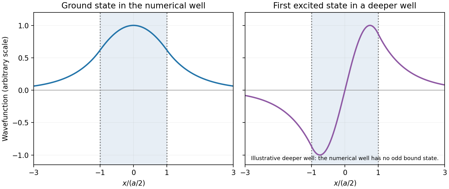
Original finite-well wavefunctions: an even nodeless ground state and an odd excited state in a deeper illustrative well
. Details. 
For the numerical well,The exterior probability of a symmetric finite-well state includes both tails:The threshold is , exceeding the well depth, so there is no excited bound state. The rounded supplied coefficients integrate to rather than exactly one; this rounding does not change the quoted probability precision materially.
A travelling wave, for example , has moving constant-phase surfaces. A standing wave, for example , has stationary nodes and can be formed from two equal counterpropagating waves.
For the half-line finite well with , define and . The hard wall requires for and , so the general allowed forms areAt the finite step both and are continuous:There is no requirement to match the derivative to zero across the infinite wall.
For a bound state , put . Normalizability excludes the growing exponential, leaving inside and outside. Matching their logarithmic derivatives givesThe exterior expression is equivalent to by rescaling its constant. Negative cotangent first occurs for ; all higher allowed intervals also have . Thus . Since , a normalizable bound state requiresThis is also sufficient: on the lowest negative-cotangent branch, the two matching sides cross whenever . The printed non-strict inequality includes the threshold limit. At equality and the exterior is not square-integrable, so it is not itself a bound state.