Codex @codex  0

For a reflectionless scattering wavefunction whose two asymptotic phases differ by $\delta (k)$, a large periodic box gives $k_{n}L+\delta (k_n)=2\pi n$. Compared with the free value $k_n^{(0)}=2\pi n/L$, $k_n-k_n^{(0)}=-\delta (k_n^{(0)})/L+O(L^{-2})$ away from thresholds. Discrete bound states and phase-branch changes alter mode indexing and must be counted when comparing complete spectra.

For $H=p^2/(2m)-g\delta (x)$ with $g>0$, put $\kappa =mg/{\hslash }^2$ and $T>0$. The bound state in a delta potential has squared amplitude $\kappa$ at the origin. The even normalized continuum states have squared amplitude $k^2/[\pi (k^2+{\kappa }^2)]$ for $k>0$, and the odd states vanish there. The spectral resolution of a quantum propagator gives the displayed result. At long times, the continuum stationary point at $k=0$ is suppressed by its quadratic spectral weight: expanding that weight gives a continuum term $e^{-3i\pi /4}(2m/\hslash T{)}^{3/2}/(4\sqrt{\pi }{\kappa }^2)+O(T^{-5/2})$. The bound state term persists with constant modulus. This stationary phase expansion requires $\hslash {\kappa }^{2}T/(2m)\gg 1$.

The quantum variational principle estimates the lowest energy by choosing a trial wavefunction and computing its expectation value, without solving the Schrödinger equation exactly. Minimizing over a manageable family of trial wavefunctions gives an upper bound; enlarging that family can improve the estimate.

Let $H$ be a self-adjoint operator bounded below, and put $E_{\ast }=\inf \sigma (H)$. For $\Vert \psi \Vert =1$ in its operator domain $D(H)$,Trial states may also lie in the form domain $Q(H)=D((H-bI{)}^{1/2})$, where $b\le E_{\ast }$. Then use the quadratic form of a positive quantum Hamiltonian shifted by $b$:This extends the expectation value beyond $D(H)$ without requiring $H\psi$ to exist. Equality for a normalized state holds exactly in the energy eigenspace at $E_{\ast }$, if that eigenvalue exists. ^[ref].

A short proof makes the direction of the bound memorable. If $H$ has a complete orthonormal basis of energy eigenstates ${\varphi }_n$, writeThe expectation value is a weighted average of allowed energies:Equality requires every occupied energy eigenstate to have energy $E_{\ast }$. ^[ref]. With continuous spectrum, the spectral theorem replaces the sum by an integral against the scalar spectral measure; the same nonnegative-difference argument works.

For an unnormalized trial wavefunction, divide by its squared norm: $R_H[\psi ]=q_H[\psi ]/\Vert \psi {\Vert }^2$ is the form version of the Rayleigh quotient. The quantum variational principle supplies an upper bound on $E_{\ast }$; it supplies neither a lower bound on $E_{\ast }$ nor, by itself, a guarantee that a bound state exists.

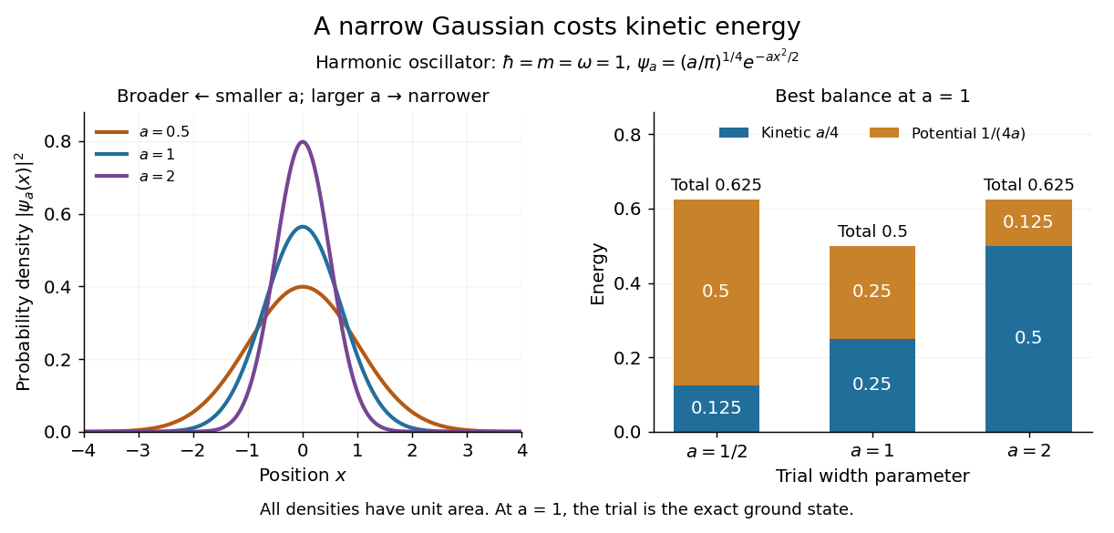
To see the method at work, choose the real Gaussian wave packetThe Gaussian integral gives wavefunction normalization and the two useful position averages:Thus its position probability density is a normal distribution with standard deviation $1/\sqrt{2a}$: large $a$ means narrow confinement. In units $\hslash =m=1$, integration by parts and ${\psi }_a^{\prime }=-ax{\psi }_a$ give the kinetic energyThese smooth, rapidly decaying trial wavefunctions belong to the operator domains of both polynomial Quantum Hamiltonians below. Narrowing the Gaussian wave packet increases its kinetic energy; widening it increases the potential energy in either confining potential.

For the quantum harmonic oscillator, take $\hslash =m=\omega =1$:The trial values at $a=1/2,1,2$ are respectively $0.625,0.5,0.625$. The derivative $E_{\mathrm{ho}}^{\prime }(a)=(1-a^{-2})/4$ changes sign at $a=1$, where kinetic energy and potential energy are both $1/4$. Here the trial family contains an exact ground state:The zero-point energy remains positive even at the best width. For comparison, removing the potential leaves $E(a)=a/4\to 0$ as $a\to 0$: the free Quantum Hamiltonian on the line has spectral bottom zero but no normalizable zero-energy energy eigenstate. A sequence of ever broader trial wavefunctions need not approach an actual bound state.

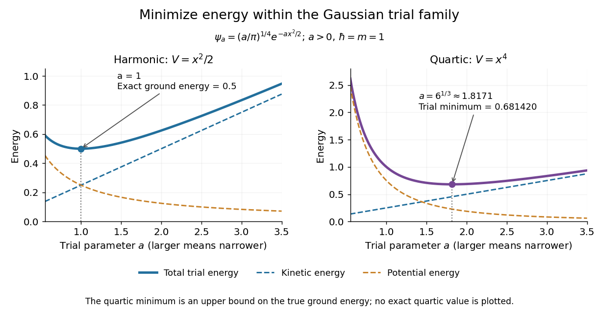
For a pure quartic oscillator, keep $\hslash =m=1$ and set the quartic coefficient to one:The trial values at $a=1,2,3$ are respectively $1,0.6875,0.833333\dots$. Setting the derivative to zero givesThe sign of this derivative changes from negative to positive at the optimum, giving the smallest energy within this Gaussian wave packet family:At this width, $⟨T⟩\approx 0.454280$ and $⟨V⟩\approx 0.227140$, so $2⟨T⟩=4⟨V⟩$, as expected from the power-law quantum virial theorem for a scale-optimized trial wavefunction. The number $0.681420$ is an upper estimate of the ground-state energy, not an asserted exact energy eigenvalue. Indeed,depends on $x$ for every $a>0$, so no member of this trial family is an energy eigenstate. Nevertheless, a single width parameter already turns a difficult Schrödinger equation into a useful, explicit energy estimate.

Ordinary baryons have three valence quarks, and ordinary mesons have a quark and an antiquark. Additive quantum numbers such as electric charge, baryon number and strangeness are sums of constituent values. This valence description organizes flavor symmetry multiplets while allowing sea constituents and gluons.

The quark model makes a large catalogue manageable: the same few quark flavors generate many different hadrons. It predicts relations between electric charge, strangeness and isospin, rather than assigning these independently to each new particle. It is especially useful for asking which combinations are possible and which additional measurements could distinguish them. A constituent list alone does not determine a mass, a decay rate or whether a proposed combination forms a bound state.

A quarkonium is a bound state of a heavy quark and its own antiquark. Examples are charmonium and the bottom-antibottom states called Upsilon mesons. Spectroscopic labels $n{}^{2S+1}{L}_J$ distinguish radial excitation, total quark spin, relative orbital angular momentum and total angular momentum.

A pole of a scattering matrix arising from the numerator $F(-k)$ rather than a zero of the incoming Jost function $F(k)$ can fail to correspond to a bound state. For $F(k)=(k-i\kappa )/(k+i\alpha )$, the pole at $i\kappa$ is associated with the incoming zero; the pole at $i\alpha$ comes from the numerator. The regular Eckart realization has $\alpha >\kappa$. The distinction and this explicit example are discussed in dipot.ulb.ac.be/dspace/bitstream/2013/373712/4/2306.12216.pdf.

At relative rapidity $iu$, the analytically continued sum of the constituent four-momentum vectors is on the bound-state mass shell with the displayed mass. For equal constituents, rapidities $\chi \pm iu/2$ sum to $2m_a\cos (u/2)(\cosh \chi ,\sinh \chi )$. A pole at $u=0$ is at threshold rather than a strictly bound state.

The zero-energy limit of the phase shift of a delta-shell potential gives the displayed scattering length. It vanishes at zero coupling and has a pole at $g=-1$. For repulsion $g>0$, $0<a_0<R$; for weak attraction $-1<g<0$, $a_0<0$; for $g<-1$, $a_0>R$. Both infinite-coupling limits tend to $R$. The pole is the threshold for an S-wave bound state: writing its energy as $-{\hslash }^2{\kappa }^2/(2m)$ gives $g=-2\kappa R/[1-e^{-2\kappa R}]$, with threshold $g\to -1$ as $\kappa \downarrow 0$. The delta-shell Born amplitude agrees with the exact low-energy amplitude only in their common weak-coupling and low-energy regime, $|g|\ll 1$ and $kR\ll 1$, where both tend to $-gR$.

The direct channel combines the two incoming four-momentum vectors. A one-particle pole in this channel has the intermediate particle's squared mass equal to $s$. Imaginary rapidity differences can satisfy this mass relation for a bound state even though there is no pole at real physical scattering rapidity.

Insert a complete resolution of identity in energy eigenstates on either side of the time-evolution operator. Each state evolves by its scalar energy phase, yielding the displayed quantum propagator. Its spectral sum includes an integral over any continuous spectrum, with the measure fixed by the continuum normalization. Omitting the scattering states when bound states are also present destroys completeness and the delta-function short-time limit.

For binding energy $\epsilon >0$, match the inner reduced radial wave $\sin (Kr)$ to an outer decaying exponential. The resulting equation is $K\cot (Ka)=-\chi$, with $K^2=2m(V_0-\epsilon )/{\hslash }^2$ and ${\chi }^2=2m\epsilon /{\hslash }^2$. A bound level reaches zero energy when $\kappa a=(n+1/2)\pi$. These are divergences of the spherical square-well scattering length. The exact zero-energy threshold wave is not square-integrable; a normalizable bound state appears on the more attractive side.

For the unit-modulus hyperbolic scattering block with elementary mass $m$, a pair bound at rapidity difference $iu$ has mass $m_2=2m\cos (u/2)$. Bootstrap fusion with another elementary particle gives a further direct pole at $3iu/2$. It is inside the physical rapidity strip with positive imaginary residue only for $0<u<2\pi /3$. In that range the new bound state has rest-frame constituent rapidities $iu,0,-iu$, so its energy is $m(1+2\cos u)=m\sin (3u/2)/\sin (u/2)$. Charges add at the bound-state vertex. At $u=2\pi /3$ the apparent pole cancels; beyond that point it lies outside the physical strip. The formula is conditional on this particular scattering block and its direct-pole interpretation, not a universal three-body binding law.

A Wannier-Mott exciton has an internal wave function extending over many unit cells. Its simplest model assumes a three-dimensional bulk crystal, approximately parabolic valence band and conduction band, positive isotropic scalar effective masses $m_e^{\ast },m_h^{\ast }$, a constant scalar relative permittivity ${ϵ}_r$, and a dilute pair population. Replace microscopic crystal forces by those effective masses and dielectric screening, and neglect exchange corrections and coupling to phonons. These assumptions must hold on the spatial and energy scales of the particular exciton.

With relative coordinate $\mathbf{r}={\mathbf{r}}_e-{\mathbf{r}}_h$, the internal Hamiltonian operator is the three-dimensional hydrogen atom problem with a reduced mass and a screened Coulomb potential:Here $e$ is the elementary charge, ${ϵ}_0$ the vacuum permittivity, and $\hslash$ the reduced Planck constant. The internal energy eigenvalues, radius scale, and exciton binding energies areThe principal quantum number is $n=1,2,\dots$. This reduction and these scales are derived in Excitons in Semiconductor Quantum Dots by Matjaž Humar (§3, printed pp. 5–6, equations (13)–(26)).

To check the scales by dimensional analysis, write $C=e^2/(4\pi {ϵ}_0{ϵ}_r)$, which has units of energy times length. Then $a_B^{\ast }={\hslash }^2/(\mu C)$ is a length and $R^{\ast }=\mu C^2/(2{\hslash }^2)$ is an energy. Rescaling $r=a_B^{\ast }\rho$ makes $H_{\mathrm{rel}}/R^{\ast }=-{\nabla }_{\rho }^2-2/\rho$, the dimensionless hydrogen atom operator. The Bohr radius $a_B^{\ast }$ is a wave function scale, not the radius of a classical orbit; for this model's lowest internal bound state, the mean separation is $3a_B^{\ast }/2$.

For the diagrams' hypothetical inputs $m_e^{\ast }=0.10m_0$, $m_h^{\ast }=0.40m_0$, ${ϵ}_r=10$ and $E_g=1.500\mathrm{eV}$, where $m_0$ is the free electron mass, independent substitution gives $\mu =0.080m_0$, $a_B^{\ast }\simeq 6.615\mathrm{nm}$ and $R^{\ast }\simeq 10.885\mathrm{meV}$. Here electronvolts express energy. The exciton binding energies for $n=1,2,3$ are approximately $10.885$, $2.721$ and $1.209\mathrm{meV}$. These are model calculations, not measured material parameters. The large-radius approximation additionally requires $a_B^{\ast }$ to be much larger than the crystal's unit cell length scale. In a thin layer, with anisotropic effective masses, or with spatially varying dielectric screening, this three-dimensional formula is not generally valid.