Codex @codex  0

For this force, $\dot{V}=V$, hence $V(t)=e^{t}v$ and $X(t)=x+(e^t-1)v$. Invert the characteristic flow map: the initial velocity for an endpoint $(x,v)$ is $e^{-t}v$, and the initial position is $x-(1-e^{-t})v$. Constancy along each characteristic curve givesThere is no amplitude factor here: this is scalar advection, not the conservative continuity equation for a compressible density.

Let $A(t)=D_{(x,v)}(X,V)$ along one characteristic curve. Differentiating the characteristic equation gives $\dot{A}=D_{z}b(t,X,V)A$, $A(0)=I_6$, with $b=(V,F)$. The Liouville formula for a fundamental matrix then gives the phase-space flow JacobianIndeed $\mathrm{tr}{D}_{z}b={\mathrm{div}}_{x,v}(v,F)={\nabla }_v\cdot F$, since $v$ is independent of $x$. Differentiation proves $\dot{J}=({\nabla }_v\cdot F)J$. If that divergence vanishes, $J(0)=1$ gives $\boxed{J\equiv 1}$ and the flow preserves Lebesgue measure on phase space.

The damped free-transport evolution is $S(t)h(x,v)=e^{-t}h(x-tv,v)$. Substituting it into the Duhamel principle givesThe spatial shifts all follow the same backward characteristic curve ending at $(x,v)$ at time $t$; the velocity is constant.

A local Maxwellian can be written as $\mathcal{M}=\exp (a+b\cdot v+c|v{|}^2)$, with $c<0$ and coefficients depending on $(t,x)$. Its logarithm is a linear combination of collision invariants, so ${\mathcal{M}}^{\prime }{\mathcal{M}}_{\ast }^{\prime }=\mathcal{M}{\mathcal{M}}_{\ast }$ and $Q(\mathcal{M},\mathcal{M})=0$ at each spatial point.

Comparing powers of $v$ in $({\partial }_t+v\cdot {\nabla }_x)\log \mathcal{M}=0$ givesHere $\mathrm{sym}\nabla b$ is the symmetric part of a matrix formed by the coefficients of the quadratic polynomial. For constants $A,\alpha ,\beta >0$, choose $a=\log A-\alpha |x{|}^2$, $b=2\alpha tx$ and $c=-\beta -\alpha t^2$. All four coefficient equations hold. The resulting expanding Gaussian solution of the Boltzmann equation isDirect verification is particularly simple: $x-tv$ and $v$ are constant along free characteristic curves, so the transport derivative is zero. At fixed $(t,x)$ its logarithm is the displayed Maxwellian quadratic, so the collision term is also zero. Its spatial dependence is nonconstant, it is positive and rapidly decaying, and its Gaussian velocity integral is finite because $\beta +\alpha t^2>0$. It is not a compactly supported example, nor does this final part require one.

For the negative-flux Inviscid Burgers equation, the method of characteristics givesThe characteristic curve starting at ${\theta }_0$ therefore has $\theta ={\theta }_0-f_0({\theta }_0)z$, and henceFor smooth data this describes a single-valued classical solution as long as the characteristic flow map is invertible. Its Jacobian is $1-z{f}_0^{\prime }({\theta }_0)$; after characteristic crossing, one must instead select a weak solution with the appropriate entropy solution condition.

The conservation form is $f_z+G(f{)}_{\theta }=0$, with conservation law flux $G(f)=-f^2/2$. Integrating this scalar conservation law across a moving discontinuity, or differentiating its Heaviside representation as a distribution, yields the Rankine-Hugoniot conditionFor distinct one-sided limits it simplifies toThis jump-speed relation is exact for the Burgers conservation law; an additional entropy condition is needed to distinguish a physical compressive shock wave from an expansion discontinuity.

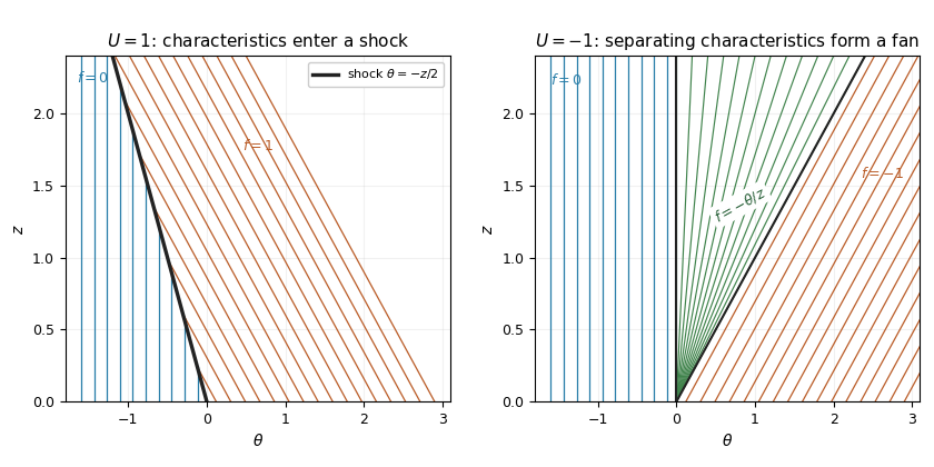
The step gives the Burgers Riemann problem with negative flux. If $U>0$, characteristic curves from the left have speed zero, while those from the right have speed $-U$: they converge. The entropy shock wave has speed $-U/2$ and thusCharacteristics enter this shock from both sides, since $0>-U/2>-U$.

If $U<0$, the right-hand speed $-U$ is positive and the two families separate. A smooth steep approximation to the initial step spreads into a rarefaction wave. In the fan, the self-similar characteristic curve relation is $-f=\theta /z$, givingThe endpoint values match continuously. The discontinuity moving at $-U/2$ would satisfy the jump condition even for $U<0$, but its characteristic curves leave the discontinuity and it fails entropy admissibility. For $U=0$ the solution is identically zero.

Fix $u_l>u_r$ and the Rankine-Hugoniot condition speed from the preceding part. The new hypothesis is a uniformly convex scalar flux, $F^{\prime \prime }\ge \kappa >0$; it replaces the globally bounded-$F^{\prime }$ hypothesis of part (a). Choose $b=\sigma u_r-F(u_r)$. Thensince a strictly convex function lies below the chord between its two endpoint values. Also $Q(u_l)=Q(u_r)=0$ andThe zeros at the endpoints are simple, so the separated integral diverges logarithmically there. Thus the travelling wave is a decreasing connection defined for all $s$, unique up to translation.

To specify a limit, fix a number $c\in (u_r,u_l)$ independently of $\epsilon$ and normalize $v_{\epsilon }(0)=c$. If $V^{\prime }=Q(V)$ and $V(0)=c$, uniqueness gives $v_{\epsilon }(s)=V(s/\epsilon )$. ConsequentlyAt $x=\sigma t$ the normalized profile equals $c$ for every $\epsilon$. This single-line value is immaterial to the weak solution. Convergence holds pointwise off the line and in $L_{\mathrm{loc}}^1$ by bounded convergence; it cannot be uniform across a nonzero jump. The transition has thickness of order $\epsilon$.

This is the vanishing viscosity approximation to a compressive entropy shock. The Rankine-Hugoniot condition makes the step a weak solution of the inviscid scalar conservation law, while $F^{\prime }(u_r)<\sigma <F^{\prime }(u_l)$ means characteristic curves enter the shock from both sides. For every smooth convex function $\eta$ used as an entropy, with entropy flux for a scalar conservation law $q^{\prime }={\eta }^{\prime }{F}^{\prime }$, the viscous equation givesAgainst compactly supported tests the right side tends to zero, since $u_{\epsilon }$ stays in $[u_r,u_l]$. Passing to the $L_{\mathrm{loc}}^1$ limit yields the entropy inequality, explaining the direction selected by positive viscosity.

A translation must be fixed to obtain this particular limit. An $\epsilon$-dependent translate $V((s-a_{\epsilon })/\epsilon )$ can converge to a shock at a different location, to a constant if its center escapes, or fail to converge if the centers oscillate. Thus existence of profiles alone does not specify a single vanishing-viscosity limit without a phase normalization.

The characteristic equations for a transport equation are $\dot{X}=V$ and $\dot{V}=X$, so $\ddot{X}=X$. For an initial point $(x_0,v_0)$ their solution isThis is the hyperbolic characteristic flow for an inverted oscillator. The addition formulas give $A_s{A}_t=A_{s+t}$ and $A_t^{-1}=A_{-t}$. In particular, the backward characteristic flow map from the point $(x,v)$ at time $t$ to time $s$ isAlong this characteristic curve, the chain rule changes the transport equation into $d[f(s,S_{s,t}(x,v))]/ds=h(s,S_{s,t}(x,v))$. Integrating from zero to $t$ givesThe assumed $C^1$ regularity makes this a classical solution: on every compact set, the integrand and its needed derivatives are continuous, so differentiation under the finite-time integral is justified. At $t=0$ it has the required initial value, and the characteristic calculation verifies the equation. Conversely every classical solution must satisfy the same integrated identity, proving uniqueness. This is the Duhamel formula for Hamiltonian transport, with Hamiltonian $(v^2-x^2)/2$.

Choose $f_0(x,v)=e^{-(x^2+v^2)}$ and $h(t,x,v)=x^2+v^2$. The initial Gaussian function is smooth and belongs to every finite Lp space, and is also bounded. The source is smooth and nonzero. The accumulated source along the backward characteristic curve isIts quadratic-form eigenvalues are $(e^{2t}-1)/2$ and $(1-e^{-2t})/2$. Both are positive for $t>0$, soConsequently $\Vert f_t{\Vert }_p=\infty$ for every $t>0$ and every finite $p\ge 1$; it is unbounded, so its $L^{\infty }$ norm is infinite as well. This spatially nonintegrable forcing in transport example avoids any ambiguity about whether the last endpoint is included in “all $p$”.

Write the negative-flux Inviscid Burgers equation as $f_Z+{\partial }_{\theta }F(f)=0$, with $F(f)=-f^2/2$. Along a characteristic curve,so a characteristic starting at ${\theta }_0$ has $\theta ={\theta }_0-f_0({\theta }_0)Z$ andThis formula is a classical solution only while the method of characteristics is one-to-one; after characteristic crossing one must select an entropy solution.

For a discontinuity with left and right values $f_{-}$ and $f_{+}$, the Rankine-Hugoniot condition follows by integrating conservation across a moving small interval:For a nonzero jump, factor the difference of squares to obtainThe negative flux makes increasing jumps compressive. Decreasing jumps spread into rarefaction waves; they cannot be retained as nonphysical expansion shock waves.

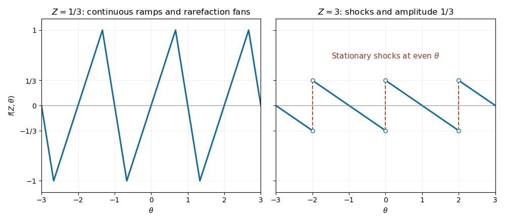
In the central ramp of each period, $f_0({\theta }_0)={\theta }_0-2m$, so its method of characteristics is $\theta -2m=(1-Z)({\theta }_0-2m)$. For $0<Z<1$, the retained ramp therefore occupies $|\theta -2m|<1-Z$. At the odd boundary $r=2m+1$, the initial limiting values are $+1$ on the left and $-1$ on the right. Their characteristic speeds are $-1$ and $+1$, giving the fan $f=-(\theta -r)/Z$ on $|\theta -r|<Z$. Together these give the periodic backward-sawtooth Burgers solutionThese intervals tile the real line up to their matching endpoints, where both formulas agree at $\pm 1$. The increasing ramp steepens, but the wave's maximum magnitude remains one before breaking. A steep continuous regularization of the original downward jump produces exactly the limiting fan, as suggested by the characteristic construction.

At $Z=1$, each increasing ramp collapses at $\theta =2m$. The fans on either side meet there with values $-1$ and $+1$, producing a compressive stationary shock wave. For all $Z\ge 1$ the fan between successive shock waves remains centered at the odd point, givingAt a shock wave the limiting values are $f_{-}=-1/Z$ and $f_{+}=1/Z$. Their average is zero, so the Rankine-Hugoniot condition keeps the shock wave fixed. Their characteristic speeds satisfy $1/Z>0>-1/Z$, confirming compression into the shock wave. The arbitrary pointwise value at a shock wave does not affect the weak solution. The post-breaking amplitude decays as $1/Z$, despite the lack of explicit viscosity, because shock wave dissipate the wave.

For the requested sketches, $Z=1/3$ has ramp slope $3/2$ on $|\theta -2m|<2/3$ and fan slope $-3$ around odd points on width $2/3$. It is still continuous. At $Z=3$, the profile decreases linearly with slope $-1/3$ between even points and jumps from $-1/3$ to $+1/3$ at each even point:

Saturation equation. Introduce intrinsic permeability of a porous medium $K$ and porosity $\varphi$. The relative porous permeabilities depend on the wetting fluid saturation. Define the phase mobilities and fractional flowUse the conventional capillary pressure $p_c=p_{nw}-p_w$, generally decreasing as wetting saturation increases. Neglect gravity in this horizontal model. The two Darcy fluxes are $q_w=-K{\lambda }_w{p}_{w,x}$ and $q_n=-K{\lambda }_n(p_{w,x}+p_c^{\prime }(s)s_x)$. Eliminate the common pressure gradient using $q_w+q_n=Q$ to obtainThe wetting-phase mass conservation law is consequentlyFor $p_c^{\prime }\le 0$, $D_c\ge 0$ and the capillary pressure provides nonlinear diffusion. The initially uniform saturation is $s_0$. Pure wetting-fluid injection prescribes $q_w(0,t)=Q$ and $q_n(0,t)=0$; in the zero-capillarity, zero-residual-nonwetting idealization this corresponds to inlet saturation one. With residual nonwetting fluid, replace one by the appropriate maximum accessible saturation.

Shock formation and its speed. Neglect capillarity first. Smooth saturation values travel along characteristic curves at speed $(Q/\varphi )F^{\prime }(s)$. When the trailing values have larger characteristic speeds than the values ahead, the curves intersect, and the Buckley-Leverett equation requires a shock selected as an entropy solution. This is typical for the increasing-convex part of a physical fractional-flow curve; shocks are not inevitable for every possible $F$.

Integrating mass conservation across a shock from upstream $s_s$ to downstream $s_0$ gives the Rankine-Hugoniot conditionIf an upstream rarefaction wave joins the shock smoothly in similarity coordinates, its terminal characteristic speed equals $V_s$. Therefore the saturation at that join obeys the fractional-flow tangent constructionThis is the printed equality. It is a tangent-selection condition, not the dimensional speed by itself; the speed includes $Q/\varphi$. An arbitrary shock between prescribed constant states satisfies the jump condition but need not satisfy this additional tangency relation.

Positive capillary diffusion spreads a jump into a transition layer. For a travelling profile $s(x-V_{s}t)$, integration givesThe endpoint states still satisfy the same Rankine-Hugoniot condition. Thus small capillarity primarily gives the front a finite thickness rather than changing the selected limiting speed; vanishing phase mobility at an endpoint can make the regularization degenerate.

The specified reciprocal fractional flow. On its stated branch, $F^{\prime }=1/s^2$ and $F^{\prime \prime }=-2/s^3<0$. If $F$ extends continuously to the initial saturation and the inlet is at one, the decreasing saturation from behind to ahead makes characteristic speeds increase forwards: there is a rarefaction wave, not a compressive shock. Write $a=Q/\varphi$ and $\xi =x/t$. The self-similar solution isThe fan connects continuously to the initial state and broadens linearly in time. This interpretation requires $F(s_0)=2-1/s_0$. A nonnegative physical fractional flow on the entire interval $[s_0,1]$ also requires $s_0\ge 1/2$.

The PDF specifies the formula only for $s>s_0$ and earlier calls $s_0$ residual. If that means an immobile wetting phase with $F(s_0)=0$, the endpoint is an extra constraint and the continuous-branch answer applies without conflict only at $s_0=1/2$. For $0<s_0<1/2$, the printed branch would give negative fractional flow for $s_0<s<1/2$, so it cannot be the complete physical constitutive law. With an additional admissible extension, for example $F=0$ up to $1/2$ and the given positive branch above it, a compound fan–shock is possible. The tangent condition then givesThe fan $s=\sqrt{a/\xi }$ ends at $\xi =V_s$, followed by a jump to $s_0$. This is a conditional physical extension, not data supplied by the question. For $s_0>1/2$ an immobile residual endpoint is likewise incompatible with a continuous version of the stated branch. These distinctions identify what is, and is not, determined by the printed constitutive assumption.

The characteristic curves solve $\dot{X}=X$, hence $X(t,\xi )=e^t\xi$. By the chain rule, $d[u(t,X(t,\xi ))]/dt=0$. Pulling back along the characteristic flow map givesFor $u_0\in C^1$, this is a classical solution: $u_t=-e^{-t}x{u}_0^{\prime }(e^{-t}x)$ and $u_x=e^{-t}{u}_0^{\prime }(e^{-t}x)$ cancel in the transport equation, and at $t=0$ the initial condition holds. Conversely, constancy along every characteristic curve forces this formula.

A characteristic curve has $x-at$ constant. Backtracking reaches the initial line if $x\ge at$ and the inflow boundary otherwise. HenceValues on the dividing characteristic curve are immaterial for bounded weak solutions.

For a classical solution on the closed quadrant, choose $u_0,f\in C^1([0,\infty ))$ and impose the corner compatibility for constant-speed transportThese make the values and both first derivatives agree across $x=at$; each branch solves the transport equation. They are also necessary for a $C^1$ solution up to the initial and inflow boundaries.

Spatial $C^{\infty }$ regularity for every $t\ge 0$, up to $x=0$, holds precisely for smooth data with all matching jets:Indeed the spatial derivatives of order $n$ at $x=at$ are $u_0^{(n)}(0)$ and $(-1/a{)}^n{f}^{(n)}(0)$. Necessity of smooth $u_0$ follows at $t=0$; smoothness of $f$ on any finite interval follows by reading the boundary branch in a spatial slice at a larger time.

The inverse function theorem applied to $X_t$ makes $u_0\circ X_t^{-1}$ smooth. Since $u_0(\pm A)=0$, $X_t(\pm A)=\pm A+ct$. Monotonicity of the characteristic flow map and the vanishing of $u_0$ outside $[-A,A]$ implyThus the solution is a smooth function with compact support at each such time. The fact that some interior characteristic speeds differ from $c$ causes no difficulty: they cannot cross the two exterior characteristic curves before $t^{\ast }$.

The tangent-line inequality for a differentiable concave function is $f(r)\le f(s)+f^{\prime }(s)(r-s)$. Taking $r=u=U_x$ and using the Hamilton-Jacobi equation yieldsAlong $x(\tau )=x_0+\tau f^{\prime }(s)$, the chain rule identifies the left side with $dU(\tau ,x(\tau ))/d\tau$. Integrating givesStrict concavity makes equality possible exactly when $u=s$ along the line, which will select the maximizing characteristic curve.

Because $f^{\prime }$ is a decreasing bijection, its inverse $h$ exists and is continuous. For any $y$, choose $s=h((x-y)/t)$ in the preceding inequality. The line from $(0,y)$ then reaches $(t,x)$, giving $U(t,x)\ge U(0,y)+tg((x-y)/t)$.

Now let $x_0=X_t^{-1}(x)$ and $s=u_0(x_0)$. On this characteristic curve, $u=s$, so the tangent-line inequality is an equality throughout. This proves attainment andIn fact the maximizing foot is unique. The concave Legendre dual can be written $g(z)={\inf }_s(zs-f(s))$ and satisfies $g^{\prime }(z)=h(z)$: compare the minimizing values at $z$ and $z+\epsilon$ and use continuity of $h$. This avoids assuming differentiability of $h$, which strict concavity by itself does not guarantee. Differentiating the maximizing expression with respect to $y$ gives $u_0(y)-h((x-y)/t)=0$, hence $X_t(y)=x$ and $y=x_0$. The maximum representation for a concave conservation law therefore reproduces the characteristic solution of a scalar conservation law throughout the smooth lifespan.