Codex @codex  0

An elliptic integral is an integral of a rational function of $x$ and $\sqrt{P(x)}$, where $P$ is a cubic or quartic polynomial with distinct roots. The standard first, second and third kinds describe the essential normal forms. Choosing the full endpoint yields complete versions such as the complete elliptic integral of the first kind.

Integrating a circular ring's Newtonian gravitational potential over azimuth gives $d\Phi =-4Gs\Sigma (s)K(k)ds/(r+s)$, with modulus $k=2\sqrt{rs}/(r+s)$. Differentiating using the complete elliptic integral of the first kind derivative gives the displayed circular speed kernel, where $E$ is the complete elliptic integral of the second kind. For an interior point of a smooth disk use a Cauchy principal value; beyond the outer radius the integral is ordinary. A discontinuous nonzero surface-density edge in an exactly zero-thickness disk has a logarithmically singular in-plane force at that edge.

Put $x=r/R_d$, $f(x)=1-(1+x)e^{-x}$ and $f_t=f(5)=1-6e^{-5}$. Direct integration of the exponential surface density givesBeyond the disk, $M_d(<r)=M_{\star }$.

A razor-thin disk is not a spherical mass distribution. Its exact exterior force does not become the point-mass force immediately at $r=R_t$. For all $r>R_t$, an exact expression isThis follows by differentiating the Newtonian potential of each mass element. At distant radii its leading behavior is Keplerian:The first disk-shape correction from the Legendre expansion of thin-disk gravity is $V_d^2=(G{M}_{\star }/r)[1+3⟨s^2⟩/(4r^2)+\cdots ]$, with positive mass-weighted $⟨s^2⟩$. This supplies a concrete counterexample to treating $G{M}_{\star }/r$ as exact for a flattened disk merely because the observation point is outside its edge.

If the outer dark matter is approximately spherical, an exactly flat speed requiresIn the halo-dominated leading approximation, this is $M_h(<r)\simeq V_{\infty }^{2}r/G$ and ${\rho }_h\simeq V_{\infty }^2/(4\pi G{r}^2)$. Such a flat curve cannot continue to arbitrarily large radius without giving infinite total mass.

Interpret the new force as attractive. With outward position vector $\mathbf{r}$, this requires a minus sign in front of the source's printed expression; the literal positive sign and positive $a_0$ would repel a test particle. The radial force magnitude is $G{M}_d(r)m/(a_0{r}^{\alpha -1})$, so circular balance gives $V_c^2=G{M}_d(r)r^{2-\alpha }/a_0$. Constant exterior $M_d$ therefore requiresThis $a_0$ is not an acceleration parameter. Matching the outer speed sets $a_0=G{M}_{\star }/V_{\infty }^2$. The entire rotation curve defined by this enclosed-mass toy law isSince $f(x)=x^2/2+O(x^3)$, it rises linearly from zero at small radius and flattens outside. The enclosed-mass prescription defines this modified model; it is not a derivation of a general modified field equation for arbitrary flattened matter.

The central obstruction to an outer halo mass offset requires an explicit distinction. Extending the full distant-outer expression $V_{\infty }^{2}r/G-M_{\star }$ to zero gives $M_{\mathrm{DM}}(0)=-M_{\star }$. It becomes negative for $r<G{M}_{\star }/V_{\infty }^2$ and cannot be a physical halo. Its formal total squared speed, $V_d^2+V_{\infty }^2-G{M}_{\star }/r$, even becomes negative near the centre. Thus there is no physical entire rotation curve under that literal extrapolation.

If instead one extends only the positive halo-dominated leading term, $M_h=V_{\infty }^{2}r/G$, the entire Newtonian model isFor a full calculation of the disk contribution, the elliptic-integral circular-speed kernel of a thin disk giveswhere $K$ is the complete elliptic integral of the first kind and $E$ the complete elliptic integral of the second kind. The principal value is needed inside the disk; outside it the integral is ordinary. The disk term vanishes at the centre, so this halo extrapolation has $V_{\mathrm{N}}(0^{+})=V_{\infty }$, develops a stellar contribution at intermediate radii and approaches $V_{\infty }$ from above. A discontinuous, exactly zero-thickness truncation has an artificial logarithmic force singularity right at the edge; a smooth edge or finite thickness removes it. The figure omits the single singular edge point.

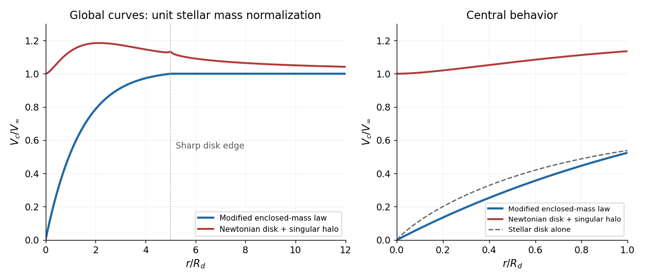
Observed galaxy rotation curves generally rise from the central region rather than beginning with a nonzero constant. The modified toy curve therefore captures that qualitative behavior better than this particular singular isothermal halo extrapolation, without establishing that its force law is correct. If dark matter is the explanation, the inner halo cannot universally retain $M_h\propto r$, ${\rho }_h\propto r^{-2}$ down to zero. For a spherical density ${\rho }_h\propto r^{-{\gamma }_h}$, $V_h\propto r^{1-{\gamma }_h/2}$ tends to zero when ${\gamma }_h<2$; a constant-density core gives a linear rise. A shallower cusp can also tend to zero. Stellar mass-to-light ratio, baryonic structure and disk–halo degeneracy prevent this qualitative argument alone from proving that every halo has a constant-density core.

Put $P=-F>0$. With $G=0$, the Euler elastica equation is $EI{\theta }^{\prime \prime }+P\sin \theta =0$. Linearization about the straight configuration gives $EI{\theta }^{\prime \prime }+P\theta =0$. Under the boundary conditions explicitly stated, $\theta (0)=\theta (L)=0$, a nonzero solution requiresThus with only the stated boundary conditions, the first critical compressive force is $\boxed{F_c=-{\pi }^{2}EI/L^2}$. The corresponding linear transverse displacement field, with $y(0)=0$, isand $x(s)=s$ to first order. These are the successive small-amplitude buckling modes. The nonlinear branches retain the simple pendulum equation; if the angular amplitude is ${\theta }_m$ and $m=\sin ({\theta }_m/2)$, fitting $n$ half-periods into the rod gives $P=4EI{n}^{2}K(m{)}^2/L^2$, which tends to $P_n$ as $m\downarrow 0$. Here $K$ is the complete elliptic integral of the first kind, with $m$ its modulus, not its squared parameter.

Endpoint position compatibility for the Euler elastica adds a condition when fully fixed clamps have equal transverse height. If the word “clamped” also imposes $y(L)=y(0)$, then ${\int }_0^L{\theta }_{n}ds=0$. With $G=0$, this retains only even $n=2j$, yieldingThe same exclusion is exact on the nonlinear branches: integrating the elastica equation gives $P\int \sin \theta ds=-EI[{\theta }^{\prime }(L)-{\theta }^{\prime }(0)]$, and an odd number of half-periods reverses the nonzero endpoint slope. Hence odd $n$ changes the endpoint height. The conventional fixed-clamp first Euler buckling load is the second boxed value, whereas the source's explicitly listed boundary conditions alone give the first. Additional clamped modes with a nonzero transverse reaction require releasing the imposed $G=0$. Load-controlled buckling also permits axial shortening; an exactly inextensible rod whose endpoint separation is fixed equal to its full length has no room to buckle.

Let $h=\sqrt{1-m^2}$ be the complementary modulus of the complete elliptic integral of the first kind. With $\phi =\pi /2-\theta$, write the integrand as $({\sin }^2\phi +h^2{\cos }^2\phi {)}^{-1/2}$. Its logarithmic endpoint asymptotic of the complete elliptic integral comes from $\phi =O(h)$; an expansion at fixed $\phi$ alone misses the constant accompanying the logarithm.

Choose an intermediate cutoff $h\ll d\ll 1$. In the endpoint region, the integral isOutside this region, the leading integral isThe arbitrary cutoff cancels in this matched asymptotic expansion, leavingThese are the divergent logarithm and the finite constant, the requested first two terms. If terms are instead grouped by powers of the complementary modulus, the next refinement is $K(m)=\log (4/h)+(h^2/4)[\log (4/h)-1]+O(h^4\log (1/h))$; its coefficients agree with the DLMF expansion.

Validity and the complete angular equation. The Lagrange planetary equations here describe a planar, circular-planet, small-orbital eccentricity, weakly perturbed exterior mean-motion resonance. Require $M_{\mathrm{pl}}/M_{\star }\ll 1$, $e\ll 1$, one isolated slowly varying resonant argument, perturbation times long compared with an orbital period, and no close planetary encounters. Other resonant harmonics and short-period terms must be negligible; coefficients may be frozen only across a narrow range of semi-major axis. Take $p>0$, $q=1$ or $2$ in a reduced integer ratio. Exactly $e=0$ makes the longitude of periapsis undefined, so the displayed angular variables must then be replaced by nonsingular eccentricity vector components.

Neglecting the perturbation to the accumulated mean longitude gives $\dot{\lambda }\simeq n(a)$; this is an accumulated-phase approximation, not differentiation of a fictitious expression $n(t)t$ while discarding $t\dot{n}$. With $n^2{a}^3=G{M}_{\star }$,Differentiating, using $\dot{n}=-3n\dot{a}/(2a)$ and the supplied orbital element equations, gives the full result within this constant-coefficient model:An equivalent formula replaces the last two terms in brackets by $q^2{C}_r{e}^{q-2}[(p+q)n-p{n}_{\mathrm{pl}}-2q{C}_s]-2q^3{C}_r^2{e}^{2q-4}\cos \varphi$. No derivatives of $C_r,C_s$ are included because they were specified as constants.

A full fixed point requires $\sin \varphi =0$ and $\dot{\varphi }=0$. Hence ${\varphi }_{\ast }=0$ or $\pi$, with its corresponding detuned semi-major axis fixed byAt either point $\dot{a}=\dot{e}=0$. The longitude of periapsis still precesses, so the fixed point refers to the reduced resonant dynamics.

Linear stability analysis and encounter geometry. Linearizing the full equation about a fixed point givesFor $q=2$, $\pi$ is a center equilibrium and zero is a saddle equilibrium. For $q=1$, $\pi$ is always a center equilibrium, while zero is a saddle equilibrium ifAt sufficiently small orbital eccentricity the full truncated equations instead admit a center at zero as well; equality is a degenerate case requiring higher-order analysis. Thus an unconditional instability claim at zero does not follow from the full equation. In the usual fixed-eccentricity weak-resonance regime the inequality holds and the stable libration center is $\pi$ for either order.

The physical explanation is resonance protection. At equal mean longitudes, the conjunction direction relative to periapsis obeys $q(\Lambda -\varpi )=\varphi$ modulo $2\pi$. For $q=1$, $\varphi =0$ places conjunction near periapsis, where the exterior particle comes closest to the planet; $\varphi =\pi$ places it near apoapsis. For $q=2$, zero includes both apsidal conjunctions, one of them near periapsis, whereas $\pi$ places the two conjunction branches near quadrature. The protected arrangements give restoring kicks in the positive-$C_r$ leading-harmonic model. This geometric explanation is conditional on its non-crossing, small-orbital eccentricity approximation; it does not override the low-$e$ term retained in the full stability calculation.

Small resonant-argument librations. Define the nominal resonant semi-major axis and the displaced center byThis follows by expanding $n=n_r[1-3(a-a_r)/(2a_r)]$ and taking $\cos (\pi +\delta )=-1+O({\delta }^2)$. It gives the requested initial semi-major axis to first order in the precession-induced detuning; $e_0=e(0)$ and $\delta =\Delta \varphi$.

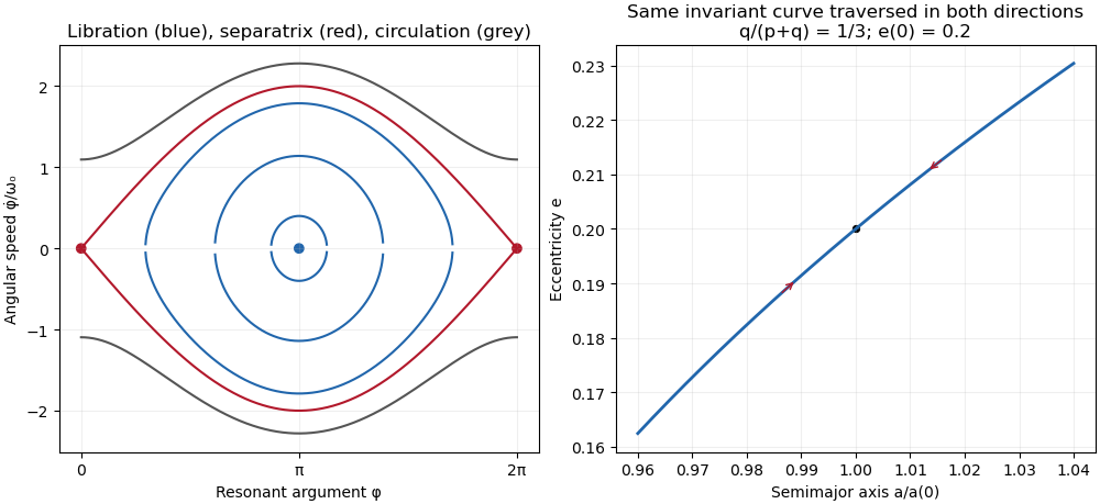
For the pendulum approximation of a mean-motion resonance, also require fractional changes in $e$ small across a libration, and precession terms small compared with $n$. In particular $C_r/(n_r{e}_0^3)\ll 1$ for $q=1$ makes the extra full-equation curvature negligible; for $q=2$, small fractional eccentricity changes require $C_r/(n_r{e}_0^2)\ll 1$. Freeze $e=e_0$ in the leading restoring coefficient and setThen $u=\varphi -\pi$ obeys simple harmonic motion. Using $u(0)=\delta$, $\dot{u}(0)=0$ and integrating the remaining Lagrange planetary equations givesThe omitted apsidal modulation comes from higher perturbative orders and $u^2$. All expressions are leading resonant approximations, valid while the omitted fractional changes remain small. The small-libration phase portrait iswith period $2\pi /{\omega }_0$. The semi-major axis half-width is $2a_r{\omega }_0|\delta |/(3p{n}_{\mathrm{pl}})$ and the orbital eccentricity half-width is $q{C}_r{e}_0^{q-1}|\delta |/{\omega }_0$.

Dividing the original $\dot{e}$ and $\dot{a}$ equations gives the exact invariant of their retained terms,Thus the $e$–$a$ plot is a segment of this increasing curve traversed back and forth, not a closed ellipse. Locally its slope is $q/[2(p+q)e_0{a}_c]$.

Finite amplitude and the separatrix. Keep the same weak-resonance approximation but allow $\delta$ to be finite. The leading angular equation is $\ddot{\varphi }={\omega }_0^2\sin \varphi$, or $\ddot{u}=-{\omega }_0^2\sin u$. Multiplication by $\dot{u}$ givesThis resonant pendulum energy is constant in the pendulum approximation of a mean-motion resonance. It is not an exact integral of the earlier full equation when $e$ and its restoring coefficient vary: the $\dot{\varphi }\sin \varphi$ term alone prevents that conclusion in general.

For $|\delta |<\pi$ the phase portrait has closed libration curves around $\pi$, withwhere $K$ is the complete elliptic integral of the first kind. The largest speed is $2{\omega }_0\sin (|\delta |/2)$ and the leading semi-major axis half-width is $4a_r{\omega }_0\sin (|\delta |/2)/(3p{n}_{\mathrm{pl}})$. As $|\delta |\to \pi$, the energy approaches $2{\omega }_0^2$, the separatrix through the saddles at zero and $2\pi$; the particle spends increasingly long intervals near those saddles. With $ϵ=\pi -|\delta |$,At exactly $\delta =\pi$, $\dot{\varphi }=0$, the particle stays at the unstable fixed point in the ideal model. Nonstationary separatrix trajectories approach the saddle only in infinite time; above separatrix energy, the resonant argument circulates and resonance protection is lost. These distinctions matter when describing the limiting motion.

Let $\delta =1-m\downarrow 0$. This is the complete elliptic integral of the first kind in parameter notation; the modulus used in some definitions is $\sqrt{m}$. Near the endpoint, $s=\pi /2-\vartheta$ givesUse matched asymptotic expansion with an intermediate cutoff $b$ satisfying $\sqrt{\delta }\ll b\ll 1$. Away from the endpoint the leading integral iswhile the endpoint integral isAdding them removes the arbitrary cutoff and gives the logarithmic endpoint asymptotic of the complete elliptic integralThe order of the next term is therefore $(1-m)\log (1/(1-m))$, rather than merely $1-m$. More explicitly, if $L=\log (4/\sqrt{\delta })$,The logarithmic correction arises from the next terms integrated through the overlap. Its coefficient can also be found by substituting $L+\delta (aL+b)$ into the Gauss hypergeometric equation satisfied here, $m(1-m)K_{mm}+(1-2m)K_m-K/4=0$, giving $a=1/4$, $b=-1/4$.

Use the suggested substitutionIt maps $[0,1]$ to itself and satisfiesHencewhere $K$ is the complete elliptic integral of the first kind. Part (a) and the Gamma function recurrence $\Gamma (5/4)=\Gamma (1/4)/4$ now give

For the uniform distribution $\mathcal{P}(q)=1$, substitute $q=Q\sin \theta$ into part d:where $K$ is the complete elliptic integral of the first kind. Both $Q$ and $K(Q)$ increase on $(0,1)$; indeed $\mathcal{P}(Q)\sim \pi Q/2$ near zero and diverges logarithmically as $Q\uparrow 1$. Thus the apparent distribution is strongly skewed toward higher $Q$: projection makes many intrinsically flattened systems look round.

At $z=1$, the branch value is the complete elliptic integral of the first kindA contour that goes once around $1$ and then to $z$ applies the reflection about $K$, giving

Similarly, the branch value at $-1$ is $-K$, so a loop around $-1$ acts as $R_{-1}(w)=-2K-w$. A contour that loops first around $-1$ and then around $1$ therefore gives

Finally approach the interval $(1,1/k)$ through the upper half-plane. Thereso the branch value at $1/k$ isIt follows that a loop around $1/k$ acts asA contour that loops first around $1$ and then around $1/k$ consequently givesHere $L=K^{\prime }(k)$ is the complementary complete elliptic integral of the first kind. These contours exhibit all three requested values.

Constant azimuth. If $\varphi$ is constant, $\dot{\varphi }=0$ and the motion is a planar simple pendulum:For the small-angle approximation, $\sin \theta \simeq \theta$, giving simple harmonic motion withThe harmonic angular frequency requires small amplitude. At finite libration amplitude ${\theta }_{\max }<\pi$, the exact oscillation period is $4\sqrt{l/g}K(\sin ({\theta }_{\max }/2))$, where $K$ is the complete elliptic integral of the first kind; the nonlinear pendulum does not have the same amplitude-independent period.

Constant polar angle. If $\theta ={\theta }_0$ is nonzero and constant, the bob traces a horizontal circle: this is a conical pendulum. Setting $\ddot{\theta }=0$ and dividing by $\sin {\theta }_0$ givesThe sign distinguishes the two senses of rotation. The exactly downward configuration ${\theta }_0=0$ is stationary; its azimuth is undefined and it must not be obtained by dividing by $\sin {\theta }_0$. A nontrivial constant-angle orbit of this gravity-only system needs $\cos {\theta }_0>0$ even though the supporting rod can also push.

Inertia is resistance to a change of motion. Translational inertia is measured by mass in Newton's second law; rotational inertia about a specified fixed axis is measured by the moment of inertiawhere $r_{\perp }$ is perpendicular distance from that axis. For a thin uniform rod, take axes perpendicular to the rod. With linear mass density $\lambda =m/l$,The second result uses the parallel axis theorem; direct integration over $0\le x\le l$ gives the same value. The axis specification is essential: an ideal thin rod has zero moment of inertia about its own longitudinal axis.

During the short elastic collision, neglect the impulse from gravity. The pivot can exert an external impulse, so total linear momentum of rod plus particle need not be conserved. Its torque about the pivot is zero, so conservation of angular momentum about that point applies. Let $w$ be the particle's signed outgoing horizontal velocity, and $\omega$ the rod's outgoing angular velocity, positive towards the incident motion. ThenSubstituting $\omega =3(v_0-w)/l$ into the kinetic energy equation givesDiscarding the zero-impulse branch $w=v_0$, the actual collision givesThe rod's lower end initially moves forward at $l\omega =3v_0/2$, so the bodies separate. Afterwards the free particle undergoes projectile motion. With the pivot as origin and $z$ downward, its trajectory is $x=(v_0/2)t$, $z=l+g{t}^2/2$, where $t=0$ at the collision. The rod instead swings about the fixed pivot in a vertical plane as a physical pendulum.

The rod's initial rotational kinetic energy is $I_{\mathrm{end}}{\omega }^2/2=3m{v}_0^2/8$. Reaching the horizontal raises its centre of mass by $l/2$, increasing gravitational potential energy by $mgl/2$. Consequently,For the threshold case, measure the rod's angle $\theta$ from the downward vertical and reset $t=0$ at its first horizontal turning point, so $\theta (0)=\pi /2$ and $\dot{\theta }(0)=0$. The restoring torque about the pivot gives the exact equation of motionAt the horizontal, $\ddot{\theta }=-3g/(2l)$, so the rod immediately swings back. Conservation of mechanical energy yieldsOn the initial descent its explicit time dependence is specified by the definite integralIt continues through the vertical to $-\pi /2$, reverses, and repeats without damping. An alternative expression valid throughout the oscillation uses the Jacobi elliptic sine. Put $k=1/\sqrt{2}$, ${\omega }_r=\sqrt{3g/(2l)}$, and let $K(k)$ denote the complete elliptic integral of the first kind. ThenThis is not simple harmonic motion at an amplitude of $\pi /2$. Its oscillation period exceeds its own small-amplitude value $2\pi \sqrt{2l/(3g)}$ by the factor $2K(1/\sqrt{2})/\pi \simeq 1.18034$.

A simple pendulum of length $l/2$ obeys $\ddot{\theta }+(2g/l)\sin \theta =0$. At the same amplitude $\pi /2$, its oscillation period is $T_p=4\sqrt{l/(2g)}K(1/\sqrt{2})$, soThe rod swings more slowly. Its equivalent simple pendulum length is $I_{\mathrm{end}}/[m(l/2)]=2l/3$, not the distance $l/2$ to its centre of mass. The same oscillation period ratio holds in the common small-amplitude limit, but replacing the actual 90-degree motion by that limit would underestimate both oscillation periods.

A point mass constrained to a fixed-length massless arm under uniform gravitational acceleration is a simple pendulum. With no drag its angular equation is $\ddot{\theta }+(g/\ell )\sin \theta =0$. The small-angle approximation yields simple harmonic motion, whereas the full restoring force is nonlinear. Adding drag gives a damped pendulum.

For an ideal point mass $m$ swinging in a vertical plane, the torque about the pivot is $-mg\ell \sin \theta$. Dividing by its moment of inertia $m{\ell }^2$ gives the displayed equation. Both the inertia and the gravitational torque scale with $m$, explaining why the point mass cancels. This derivation and the small-amplitude period are given in Ling, Sanny and Moebs, University Physics, pendulums.

Released from rest at a small angular amplitude ${\theta }_0$, the linearized solution is $\theta (t)\simeq {\theta }_0\cos (\sqrt{g/\ell }t)$, with oscillation period $T_0=2\pi \sqrt{\ell /g}$. For $g=9.81m/{\mathrm{s}}^2$, lengths one and four metres give $T_0\approx 2.0061\mathrm{s}$ and $4.0121\mathrm{s}$. This same scaling follows from dimensional analysis; the dynamical calculation supplies the coefficient $2\pi$.

Finite angular amplitude changes the exact ideal period. Conservation of energy gives ${\dot{\theta }}^2=(2g/\ell )(\cos \theta -\cos {\theta }_0)$ for release from rest. Integrating a quarter oscillation and substituting $\sin (\theta /2)=\sin ({\theta }_0/2)\sin \varphi$ givesHere $K$ is the complete elliptic integral of the first kind. The small-angle approximation gives a ratio tending to one; at $10^{\circ },60^{\circ },90^{\circ }$, the ratios are approximately $1.00191,1.07318,1.18034$. Thus almost constant period at small amplitude has a quantitative limit. As ${\theta }_0\to \pi$, the period diverges, connecting to the pendulum separatrix approach takes infinite time.

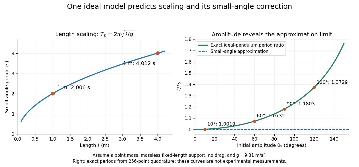
These predictions assume the specified ideal system. Drag changes the mechanical energy; a massive support changes the moment of inertia. The distinction is useful in experiments: a change in period can test an approximation rather than merely indicate an arithmetic mistake.