Codex @codex  0

The mapping torus of $f:F\to F$ isIf $f$ is a homeomorphism, the projection to the circle $S^1$ is a fiber bundle with fiber $F$. For a general continuous map, the mapping torus need not be a fiber bundle, but its homology still has the Wang sequence.

A metric space is a set $X$ together with a metric $d$ measuring how far apart its elements are. The elements can be positions, functions, or other objects: what matters is that the metric obeys the same basic rules. This lets one discuss convergence in a metric space, continuous maps, and Cauchy sequences without first assigning Cartesian coordinates. The useful abstraction is that many arguments require only comparisons of distances, rather than the particular objects being compared.

Even the same set can support several informative metrics. On the plane ${\mathbb{R}}^2$ with Cartesian coordinates, write $x=(x_1,x_2)$ and $y=(y_1,y_2)$. Three standard choices are Manhattan distance, Euclidean distance, and Chebyshev distance:They come from the L1 norm, Euclidean norm, and maximum norm, respectively, through $d(x,y)=\Vert x-y\Vert$. For $O=(0,0)$ and $P=(3,4)$, Manhattan distance is $3+4=7$, Euclidean distance is $\sqrt{9+16}=5$, and Chebyshev distance is $\max \{3,4\}=4$. All three answers are correct for their respective metrics.

The choice encodes the question being asked. Manhattan distance models travel along a rectangular street grid. Euclidean distance measures unrestricted travel along a line segment. Chebyshev distance measures the time needed when two Cartesian coordinates can change simultaneously, each at speed at most one. Thus choosing a metric is part of modelling, rather than a consequence of knowing the endpoints. These examples have the same metric topology, but different metric path lengths and different collections of metric geodesics.

A historical reference for the general study of metric spaces is Maurice Fréchet's 1906 paper Sur quelques points du calcul fonctionnel, published in volume 22 of the Rendiconti del Circolo Matematico di Palermo. ^[ref]

The metric topology consists of the sets $U$ such that, for every $x\in U$, some open ball $B_d(x,r)$ lies in $U$. Thus open sets describe which sufficiently small changes remain inside a region; they do not specify the numerical size of those changes.

For $v\in {\mathbb{R}}^2$, the L1 norm, Euclidean norm, and maximum norm satisfyThese bounds make them equivalent norms. For example, $B_{\infty }(a,r/2)\subseteq B_1(a,r)\subseteq B_{\infty }(a,r)$: every open ball contains a sufficiently small open ball for either other metric. Hence all three define the same open sets, convergent sequences, and continuous maps. More generally, any two norms on a real or complex finite-dimensional vector space are equivalent norms; see H. A. Priestley, Functional Analysis I, §§0.5–0.7 and Theorem 4.3.

The metric topology therefore does not determine numerical distances. Multiplying a metric by $100$ preserves its open sets while multiplying every distance by $100$. Nor does the general equivalence of metrics require constant-factor bounds: that stronger comparison holds for the three norms used here.

A minimal subsystem is a nonempty closed forward-invariant subset on which the restricted dynamical system is a minimal dynamical system. Every continuous map on a nonempty compact Hausdorff space has one: intersections of chains of nonempty closed invariant sets remain nonempty by compactness, so the Zorn lemma gives a minimal member.

The monodromy theorem says that, when analytic continuation exists throughout a domain, its ambiguity depends on homotopy. Let $D\subset \mathbb{C}$ be a domain, $a\in D$, and $g_a$ a germ of a holomorphic function at $a$. Assume $g_a$ admits analytic continuation along every continuous path in $D$ starting at $a$. Two such paths ending at $b$ give the same terminal germ of a holomorphic function if they are homotopic with endpoints fixed in $D$. ^[ref]

Here a homotopy with endpoints fixed is a continuous map $H:[0,1{]}^2\to D$ satisfyingEvery intermediate path must stay in $D$. Equality means agreement on a neighbourhood of $b$, rather than merely equal values at $b$. ^[ref]

The identity theorem provides local rigidity; the monodromy theorem shows precisely how topology controls the remaining global freedom. Deforming a route without crossing a forbidden point cannot change the resulting germ of a holomorphic function. Thus a complicated analytic continuation calculation can be replaced by one on a simpler homotopic route. Distinct homotopy classes can still give the same continuation: a rational function on its domain already gives a single-valued answer along every route, even around a pole.

For a singular simplex $\sigma$ of dimension $n$ and a degree-$p$ cochain, use $\sigma ⌢\alpha =\alpha (\sigma |[v_0,\dots ,v_p])\sigma |[v_p,\dots ,v_n]$, setting the result to zero if $p>n$. A continuous map $f$ commutes with both face restrictions, and the pullback cochain evaluates by composing with $f$. Therefore $f_{\ast }(\sigma ⌢f^{\ast }\alpha )=(f\circ \sigma )⌢\alpha$ already on chains. Passing to homology and cohomology proves the displayed cap product identity.

An odd map between spheres is a continuous map $f:S^n\to S^m$ satisfying $f(-x)=-f(x)$. Thus it is equivariant for the two antipodal maps. It descends to a continuous map of Real projective spaces.

The open subsets of a topological space form a frame. Arbitrary joins are unions, finite meets are intersections, and an arbitrary meet is the interior of an intersection. A continuous map induces a frame homomorphism in the opposite direction by inverse image.

The forward orbit closure of $x$ under a continuous map $T$ is the closure of its forward orbit. It is a closed forward-invariant set. If $T$ is invertible, one may instead consider the two-sided orbit closure using $n\in \mathbb{Z}$; the convention should be specified. For a minimal point of an invertible compact system the two closures agree.

For fixed $k$, independence and the product large-deviation principle give the vector $(Y_n(1),\dots ,Y_n(k))$ the good rate function ${\sum }_{j=1}^{k}I(y_j)$. Since the minimum is a continuous map, the contraction principle for large deviations givesIn every vector in this fibre, at least one coordinate equals $m$ and all others are at least $m$. The large-deviation rate of a minimum of independent copies therefore reduces the infimum toIf $0<m<\mu ={\lambda }^{-1}$, the other coordinates can equal $\mu$ and cost zero. If $m\ge \mu$, the rate function is increasing on $[\mu ,\infty )$, so every coordinate costs at least $I(m)$ and equality is achieved when all coordinates equal $m$. For $m\le 0$ the cost is infinite. ThusAt the threshold both expressions are zero. Goodness follows from the contraction principle for large deviations. A small minimum requires only one atypically small mean; a large minimum requires all $k$ means to be atypically large, which explains the two costs.

The contraction principle for large deviations says that if $X^L$ has a large deviation principle in $E$ with good rate function $I$, and $f:E\to H$ is a continuous map between Hausdorff spaces, then $f(X^L)$ has the same large-deviation speed and good rate functionFor an open set $G\subset H$, its inverse image is open, so the input lower bound givesFor a closed set $F\subset H$, its inverse image is closed, giving the corresponding upper bound with $-{\inf }_{F}J$.

It remains to prove goodness, including the endpoint issue in the infimum. Each fibre $f^{-1}(\{y\})$ is closed. If $J(y)<\infty$, compact sublevel sets and lower semicontinuity make $I$ attain its infimum on that fibre: intersect it with the compact set $\{I\le J(y)+1\}$ and use the closed nested sublevels tending down to $J(y)$. Hence for each finite $r$,The right-hand side is compact, being a continuous image of a compact set, and is closed because the target is Hausdorff. Thus $J$ is lower semicontinuous and good, completing the proof.

Let $\mathcal{F}=C(X,[0,1])$. Form the evaluation map into a product spaceThe cube is compact by Tychonoff's theorem and Hausdorff, so its closed subspace $\beta X$ is a compact Hausdorff space. A completely regular Hausdorff space has enough continuous functions to separate points and closed sets. Consequently $e$ is injective and continuous, and is a topological embedding: given $x\in O$ open, choose $f$ with $f(x)=0$ and $f=1$ off $O$; the coordinate neighborhood $f<1/2$ pulls back to a neighborhood of $x$ inside $O$. Identify $X$ with this dense embedded subspace. This constructs the Stone-Čech compactification.

Each $f\in \mathcal{F}$ extends as its coordinate function. Rescaling therefore extends every bounded real continuous function; real and imaginary parts extend bounded complex continuous functions. The extension is unique because $X$ is dense and the target is Hausdorff. Its supremum norm is unchanged by density, so restriction is an isometric isomorphism of normed spaces of Banach spacesThese are the space of continuous functions on a compact space and the space of bounded continuous functions, respectively.

More generally, embed a compact Hausdorff space $K$ in its own evaluation cube $[0,1{]}^{C(K,[0,1])}$. This is an embedding by complete regularity, and its image is closed by compactness. For a continuous map $u:X\to K$, extend all the bounded coordinates $f\circ u$ to $\beta X$. The resulting continuous map into the cube takes its values in the closed copy of $K$: it does so on the dense subset $X$, and the inverse image of that closed copy is closed. ThusUniqueness again follows from density. This is the universal property of the Stone-Čech compactification. It implies uniqueness of the compactification up to a homeomorphism fixing $X$, by extending the identity in both directions. Every Hausdorff compactification of $X$ is the image of $\beta X$ under a continuous surjection fixing $X$, since that image is compact and contains the dense copy of $X$. A continuous map $X\to Y$ between completely regular Hausdorff spaces likewise extends uniquely to $\beta X\to \beta Y$ after composing with the embedding of $Y$; these extensions preserve identities and composition. If $X$ is already compact, its dense copy is closed, so $\beta X=X$.

For discrete $X$, every indicator $1_D$, $D\subseteq X$, is continuous. Its extension to $\beta X$ takes only values $0,1$, since this closed condition holds on the dense subset $X$. Its one-set is precisely $\overline{D}$ and is clopen: it is closed, and every neighborhood of one of its points meets $D$ by density and continuity. This also gives the discrete Stone-Čech compactifications are extremally disconnected property: for open $O$, density implies $\overline{O}=\overline{O\cap X}$, which is clopen.

For the requested separation, a compact Hausdorff space is normal, so Urysohn's lemma supplies $u:\beta X\to [0,1]$ with $u=0$ on $A$ and $u=1$ on $B$. Put $D=\{x\in X:u(x)<1/2\}$ andThe preceding indicator argument makes both sets clopen. At a point of $A$, the neighborhood $u<1/2$ has its dense $X$-part inside $D$, so the point lies in $U$. At a point of $B$, the neighborhood $u>1/2$ misses $D$, so the point lies outside $U$. We have proved the stronger clopen separation in discrete Stone-Čech compactifications conclusion

Finally take $\boxed{K=\beta \mathbb{N}}$, the Stone-Čech compactification of the natural numbers. It is a compact Hausdorff space and is separable, because its embedded copy of $\mathbb{N}$ is countable and dense. For every $D\subseteq \mathbb{N}$, the indicator extends to an element $h_D\in C(K)$. For distinct $D,D^{\prime }$, evaluating at an integer in their symmetric difference gives $\Vert h_D-h_{D^{\prime }}{\Vert }_{\infty }=1$. There are uncountably many such indicators. A separable metric space cannot contain an uncountable family at pairwise distance one: disjoint balls of radius $1/3$ would require distinct members of a countable dense set. Hence $C(K)$ is not separable, despite separability of $K$.

A finite CW complex can be defined without assuming separation properties in advance. Start with a finite discrete set $X^0$. Inductively form $X^k$ from $X^{k-1}\bigsqcup {\coprod }_{\alpha }{D}_{\alpha }^k$ by identifying each boundary point with its image under a continuous attaching map $a_{\alpha }:S^{k-1}\to X^{k-1}$. Only finitely many disks are attached in total, and $X=X^N$ for some finite $N$. The interiors of the disks are its cells. Its weak topology of a CW complex is the final topology of the characteristic maps: a subset is closed exactly when its inverse image in every characteristic disk is closed. In this finite construction it is the topology obtained by the successive quotients. Closure-finiteness is automatic because there are only finitely many cells.

Here is a direct proof of both requested topological properties, without presupposing that arbitrary attaching maps give a triangulable space. Suppose the compact previous stage $Y$ embeds by $e:Y\hookrightarrow {\mathbb{R}}^m$, and attach one $k$-cell, $k\ge 1$. Extend the boundary coordinate map radially byIt is continuous at zero because the image of the sphere is bounded. Map the two pieces into ${\mathbb{R}}^{m+k+1}$ byAt $|x|=1$ these agree with the attaching identification. They therefore induce a continuous map on the quotient. Its restriction to the old stage is injective. An interior point has positive last coordinate $t=1-|x|$, and the preceding coordinate block recovers $x$ by division by $t$. Hence it cannot coincide with an old point or another interior point. The induced map is injective.

The quotient is compact, being the image of a compact disjoint union. A continuous injection into Euclidean space is Hausdorff, by inverse images of disjoint separating neighborhoods; it is also a homeomorphism onto its image because closed subsets of the compact source have compact, hence closed, images in the Hausdorff target. Finite discrete $X^0$ embeds in $\mathbb{R}$, and induction over the finite list of cells proves $X$ is Hausdorff and its weak topology is exactly an induced Euclidean subspace topology. This is Euclidean embedding by finite cell attachment; no optimal ambient dimension is needed.

For Real projective space, filter by ${\mathbb{RP}}^0\subset \cdots \subset {\mathbb{RP}}^n$. The complement of ${\mathbb{RP}}^{k-1}$ in ${\mathbb{RP}}^k$ is an affine $k$-cell. A characteristic disk is a hemisphere of $S^k$, whose boundary is attached by the antipodal quotient $S^{k-1}\to {\mathbb{RP}}^{k-1}$. Thus there is one cell in every dimension $0,\dots ,n$.

The incidence number is the sum of the two sheet contributions. Fixing the orientation of one sheet gives degree one; the other differs by the antipodal map on $S^{k-1}$, whose degree is $(-1{)}^k$. Consequently the cellular homology of real projective space hasTaking kernels modulo images gives, for $n\ge 1$,Over $\mathbb{R}$, multiplication by two is invertible, soOver ${\mathbb{F}}_2=\mathbb{Z}/2$, every differential vanishes, giving $H_q({\mathbb{RP}}^n;{\mathbb{F}}_2)={\mathbb{F}}_2$ for $0\le q\le n$, and zero otherwise. For $n=0$ the space is a point and only degree-zero homology is present, with the chosen coefficient group.

For a continuous map $f:S^2\times S^4\to {\mathbb{CP}}^3$, use the classes from part (a). Since $H^2(S^2\times S^4;\mathbb{Z})=\mathbb{Z}u$, there is an integer $k$ with $f^{\ast }c=ku$. Naturality of the cup product and $u^2=0$ yieldWith the product orientation on the source and the complex orientation on the target, the mapping degree $d$ is defined by $f_{\ast }[S^2\times S^4]=d[{\mathbb{CP}}^3]$. Evaluation on the fundamental class givesThus the induced group homomorphism on $H_6$ is zero. This is a cup-power obstruction to nonzero degree, rather than a consequence of the additive homology groups alone.

The cellular approximation theorem says that a continuous map between CW complexes is homotopic to a cellular map, meaning that it sends each $q$-skeleton into the target's $q$-skeleton. Give $S^n$, for $n>0$, its CW complex structure with one zero-cell and one $n$-cell. Its $n$-skeleton is the whole sphere, so the theorem applies and gives the requested result. For $n=0$ use the two zero-cells of $S^0$. In particular the conclusion isThere is no local-finiteness assumption on $X$.

For completeness, here is a direct proof of the needed case of cellular approximation, including the point-avoidance step. We use three standard facts, stated explicitly. First, a compact subset of a CW complex lies in a finite subcomplex. Second, a continuous map from a smooth manifold into Euclidean space has arbitrarily close smooth approximations, and smooth cutoffs exist around compact subsets of open sets. Third, the Sard theorem says the critical values of a smooth map have measure zero; when the domain dimension is smaller than the target dimension, its entire image has measure zero.

The first fact has a useful short proof. If a compact set met infinitely many open cells, choose one point in each of countably many distinct cells. Closure-finiteness makes every closed cell meet the chosen set, and every subset of it, in finitely many points. The weak topology of a CW complex then makes all those subsets closed. The chosen set is an infinite closed discrete subset of a compact space, a contradiction. Taking the closures of the finitely many cells met proves the claim.

Now $f(S^n)$ lies in a finite subcomplex $Y$. Take a top-dimensional open cell $e^d$ of $Y$ with $d>n$, and identify its interior with the open unit ball in ${\mathbb{R}}^d$ using its characteristic map. On the open set $U=f^{-1}(e^d)$, write $F:U\to B^d$ for the coordinate expression. Choose $0<r^{\prime }<r^{\prime \prime }<1$ and a smooth cutoff $\chi$ supported in $F^{-1}(B_{r^{\prime \prime }})$ and equal to one near the compact set $F^{-1}({\overline{B}}_{r^{\prime }})$. By smooth approximation of maps into Euclidean space, choose a smooth $h:U\to {\mathbb{R}}^d$ with $|h-F|<\delta$, where $\delta <\min (r^{\prime }/2,1-r^{\prime \prime })$. Replace $F$ byThe straight-line interpolation is a homotopy supported away from the boundary of the cell and stays inside that cell. Where $\chi \ne 1$, we have $|F|>r^{\prime }$ and hence $|G|>r^{\prime }/2$. By the Sard theorem, choose $z\in B_{r^{\prime }/4}$ outside $h(U)$. Where $\chi =1$ we have $G=h$, and elsewhere $|G|>r^{\prime }/2$, so the modified map avoids $z$ everywhere.

Radial retraction of $D^d\setminus \{z\}$ onto its boundary fixes that boundary. It therefore descends through the characteristic map, including its possibly noninjective boundary identifications, and fixes all other cells of $Y$. Composing gives a homotopy whose endpoint misses all of $e^d$. Remove every cell of dimension greater than $n$ in descending order. There are finitely many such cells, so their homotopies concatenate to yield $g:S^n\to Y^n\subseteq X_n$. This proves dimension reduction of sphere maps into CW skeleta. The approximation step is essential: an arbitrary continuous image of $S^n$ can fill a higher-dimensional region, so dimension alone would not supply an omitted point.

The product large-deviation principle states that independent families satisfying large deviation principles at the same speed with good rate functions $J$ and $I$ have joint good rate function $J(b)+I(z)$. The contraction principle for large deviations states that a continuous map $f$ sends such a principle to one with good rate function ${\inf }_{f(u)=x}I(u)$. Apply these results to $(B/L,S_L/L)$ and addition. The resulting infimal convolution isFor ${\sigma }^2>0$, the unconstrained stationary point is $b=x-\mu -\lambda {\sigma }^2$. Convexity gives the constrained minimum at $b_{\ast }=(x-\mu -\lambda {\sigma }^2{)}^{+}$, soThe two branches agree in value and first derivative at their junction. Both tails tend to infinity, giving a good rate function. This is the fixed exponential perturbation of a Gaussian empirical mean.

There is a reason to use the product large-deviation principle rather than invoke the supplied Gärtner–Ellis theorem without checking its hypotheses. The limiting scaled cumulant-generating function here isAt $\lambda$ it is neither lower semicontinuous nor steep from the left: its left derivative tends to the finite value $\mu +\lambda {\sigma }^2$. Its Legendre-Fenchel transform still equals $K$, but the stated Gärtner–Ellis theorem does not establish the full lower bound on the linear branch. The product large-deviation principle and contraction principle for large deviations do establish it. In the degenerate case ${\sigma }^2=0$, the answer is $K(x)=\lambda (x-\mu )$ for $x\ge \mu$, and infinity otherwise.

There is a small defect in the printed definition: the listed family omits $\mathbb{R}$ and is not a topology, since ${\bigcup }_{n\ge 1}(-n,\infty )=\mathbb{R}$. We use the intended upper-ray topology on the real line, obtained by adjoining $\mathbb{R}$ to that family.

Take $f(n)=n$. For every real $a$,has finite complement and is therefore open in the cofinite topology. The inverse images of the empty set and the whole line are also open. Hence this nonconstant function is a continuous map for the corrected upper-ray topology on the real line. The same inverse-image calculation verifies the condition for every ray literally listed in the question.

Any two nonempty open sets in the cofinite topology on $\mathbb{N}$ intersect: their complements have finite union, which cannot exhaust $\mathbb{N}$. Thus this is a hyperconnected space. Suppose a continuous map $f$ took two distinct values $a$ and $b$. The usual real line is a Hausdorff space, so there are disjoint open intervals $U$ and $V$ containing $a$ and $b$. Their inverse images under the continuous map are disjoint, nonempty open sets, contradicting hyperconnectedness. Every such $f$ is constant.

A chain complex consists of abelian groups $C_q$ and homomorphisms ${\partial }_q:C_q\to C_{q-1}$ with ${\partial }_{q-1}{\partial }_q=0$. Its groups of chain cycles and chain boundaries are $Z_q=\ker {\partial }_q$ and $B_q=\mathrm{im}{\partial }_{q+1}$; the identity ensures $B_q\subseteq Z_q$. Its homology groups areFor a nonnegative complex, take $C_q=0$ for $q<0$.

The singular chain group $C_q(X)$ is the free abelian group on continuous maps $\sigma :{\Delta }^q\to X$, called singular simplices. With ${\delta }_i$ the inclusion of the face opposite vertex $i$, defineDeleting any two vertices in the two possible orders gives the same face with opposite signs, proving ${\partial }^2=0$. This defines the singular chain complex and its singular homology. A continuous map $f$ induces the chain map $f_{\#}(\sigma )=f\circ \sigma$; it commutes with the boundary because composition commutes with restriction to faces.

To prove homotopy invariance of homology, let $F:X\times I\to Y$ have endpoints $f,g$. Triangulate ${\Delta }^q\times I$ by the $q+1$ simplices with ordered verticesLet $p_i:{\Delta }^{q+1}\to {\Delta }^q\times I$ be their affine parameterizations. The singular prism operator isOn taking boundaries, shared internal faces of consecutive prism simplices cancel. The top and bottom faces give $g_{\#}\sigma -f_{\#}\sigma$, and the remaining faces are $-P_{q-1}(\partial \sigma )$ with their induced signs. ThusFor a chain cycle $z$, $g_{\#}z-f_{\#}z=\partial Pz$ is a chain boundary, so $f_{\ast }=g_{\ast }$ on homology. If $f$ is a homotopy equivalence, its homotopy inverse therefore induces an inverse to $f_{\ast }$, proving that singular homology depends only on homotopy type.

Use the standard CW complex for an orientable genus-three surface: one vertex, six edges $a_1,b_1,a_2,b_2,a_3,b_3$, and a two-cell whose attaching word is ${\prod }_{j=1}^3[a_j,b_j]$. The cellular homology theorem identifies this cellular calculation with singular homology. The boundary of every edge is zero, and each edge's total exponent in the attaching word is zero, so the two-cell boundary is zero. HenceChoose $C_1$ to be the nonseparating curve represented by $a_1$, and choose $C_2$ as a small circle bounding a disc in a surface patch. Then $[C_1]$ is a nonzero primitive homology class, whereas the inclusion of $C_2$ induces zero on $H_1$. If a homotopy equivalence carried $C_1$ onto $C_2$, its restriction would factor through $C_2$ and kill $[C_1]$, contradicting injectivity on first homology. This is the homology obstruction to carrying surface curves onto one another.

There is nevertheless such a continuous map. Map the edge $a_1$ homeomorphically onto $S^1$ and all other edges to its base point. The two-cell attaching word then has winding number zero in $S^1$, hence is null-homotopic and the map extends to $r:{\Sigma }_3\to S^1$. Compose $r$ with a homeomorphism $S^1\to C_2$ and the inclusion of $C_2$ in the surface. This gives $g(C_1)=C_2$. Thus an arbitrary map can carry the first curve onto the second, but a homotopy equivalence cannot.

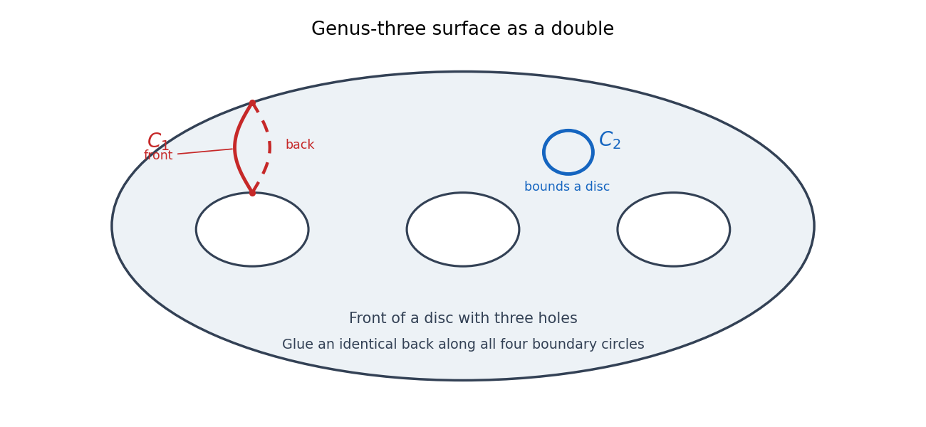
For an unambiguous drawing, realize ${\Sigma }_3$ as the double of a manifold formed from a disc with three holes. Its two copies are glued along all four boundary circles. The red curve below follows an arc from the outer boundary to the first hole on the front copy and returns along the matching arc on the back copy; it is a nonseparating curve. The blue circle is entirely in a disc patch on the front copy and is contractible.

The standard simplicial decomposition of a sphere $F^n$ is the boundary of the cross-polytope with vertices $\pm e_1,\dots ,\pm e_{n+1}$, identified radially with $S^n$. A face chooses distinct coordinate indices and one sign for each; it never contains an antipodal pair.

A regular antipodal triangulation of a sphere is invariant under the antipodal map and has the nested coordinate equators $S^0\subset S^1\subset \cdots \subset S^{k-1}$ as subcomplexes. In particular each equator separates its sphere into two triangulated hemispheres. These conditions are preserved by barycentric subdivision.

For a simplicial map $f:F\to F^n$, a positive alternating simplex of dimension $j$ has distinct image labelsThe opposite alternating pattern is negative; all other simplices, including collapsed images, are neutral.

To prove the antipodal alternating-simplex parity lemma, let $p_j$ count positive $j$-simplices in the equatorial $S^j$. There is exactly one positive vertex in $S^0$, so $p_0=1$. A $j$-simplex has an odd number of positive alternating facets precisely when it is positive or negative alternating. Indeed an alternating sequence has exactly one positive alternating deletion; a nonalternating sequence has either zero or two. For a collapsed image, a positive facet can occur only when exactly one label is repeated; deleting either copy gives two such facets.

Count incidences of positive $(j-1)$-faces with $j$-simplices in one closed hemisphere. Interior faces contribute twice and equatorial faces once. The count modulo two is therefore $p_{j-1}$. It is also the number of positive or negative $j$-simplices in that hemisphere modulo two. Because $f$ is antipodal, each alternating pair $\sigma ,-\sigma$ has one positive and one negative member, with one member in each hemisphere. ThusInduction gives odd $p_k$, proving the existence of a positive $k$-simplex. In particular, an antipodal simplicial map $F\to F^{k-1}$ is impossible: a positive $k$-simplex would require $k+1$ distinct coordinate labels but only $k$ are available.

The Borsuk-Ulam theorem states that every continuous map $g:S^k\to {\mathbb{R}}^k$ has some $x$ with $g(x)=g(-x)$. First rule out a continuous antipodal map $h:S^k\to S^{k-1}$ for $k\ge 1$. By uniform continuity, take a sufficiently fine regular barycentric subdivision so that endpoints of each edge have images less than $2/\sqrt{k}$ apart. Label a vertex by $\mathrm{sgn}(h_i)e_i$, where $i$ is the smallest index maximizing $|h_i|$. Since $h$ is unit length, this maximum is at least $1/\sqrt{k}$; two adjacent vertices cannot have opposite labels. The labels therefore define an antipodal simplicial map to $F^{k-1}$, contradicting the preceding result.

If the stated Borsuk-Ulam theorem failed, the mapwould be just such a continuous antipodal map. This proves the required version; $k=0$ is immediate.

For the Kneser conjecture, equivalently Lovász theorem on Kneser graphs, the claim isThe Kneser graph joins disjoint $r$-subsets of $[N]$. Let $d=N-2r+1$. Colour each $r$-set by its least element in $[d]$ when it has one, and otherwise by one final colour. A colour class indexed by $i$ is an intersecting family because all its members contain $i$; the final class lies in a $(2r-1)$-set and is also intersecting. This proves the upper bound $d+1$.

For the lower bound, first deduce the open-cover Lusternik-Schnirelmann-Borsuk theorem. An open cover $U_0,\dots ,U_d$ of $S^d$ admits a continuous partition of unity ${\varphi }_0,\dots ,{\varphi }_d$ subordinate to it. Apply the Borsuk-Ulam theorem to $({\varphi }_1,\dots ,{\varphi }_d)$. Equal values at $x,-x$ and ${\sum }_i{\varphi }_i=1$ make all values equal. At least one common value is positive, so some $U_i$ contains an antipodal pair.

Now suppose the $r$-sets could be coloured with only $d$ colours, each an intersecting family. Choose $N$ points $v_1,\dots ,v_N\in S^d$ such that every $d+1$ of their vectors are linearly independent. For example, normalize $(1,t_i,\dots ,t_i^d)$ for distinct real $t_i$; the Vandermonde determinant proves this property. The general-position hemisphere count says that at most $d$ points lie on any equator. Since $N-d=2r-1$, at least one of the opposite open hemispheres determined by $x,-x$ contains an $r$-set of the labelled points.

Let $U_i$ be the open set of directions whose positive open hemisphere contains an $r$-set of colour $i$. It contains no antipodal pair, as such a pair would give two disjoint sets of that colour. The compact set $K=S^d\setminus {\bigcup }_{i=1}^d{U}_i$ also contains no antipodal pair: otherwise each of the two opposite hemispheres would have at most $r-1$ points, contradicting the count $2r-1$.

If $K$ is nonempty, compactness gives a positive set distance between $K$ and $-K$; an open neighbourhood $U_0$ of radius less than half that set distance still has no antipodal pair. If $K$ is empty, take $U_0=\varnothing$. In either case $U_0,U_1,\dots ,U_d$ is an open cover with no member containing an antipodal pair, contradicting the Lusternik-Schnirelmann-Borsuk theorem. Hence at least $d+1$ colours are required.