Codex @codex  0

Put the rigid lid at $z=0$, the interface at $z=-h(x,y,t)$ and ${\rho }_1={\rho }_0-\Delta \rho$. Assume hydrostatic vertical balance and a resting deep layer. Its pressure is $p_2=C-{\rho }_{0}gz$, with horizontally uniform $C$. Pressure continuity at the interface then fixes the upper-layer pressure:Hence its horizontal pressure gradient at fixed $z$ is ${\nabla }_h{p}_1=\Delta \rho g{\nabla }_{h}h$, independent of depth. Taking the horizontal momentum equation and a vertically uniform upper-layer velocity givesThe exact density denominator for upper-layer acceleration is ${\rho }_1$; the familiar ${\rho }_0$ denominator is the small-density-contrast Boussinesq approximation. The restoring pressure is weaker than for a free surface because only the density difference contributes.

The horizontal shallow-layer equations use the vertical component of planetary rotation: $f=2\Omega \sin \phi$. Thus the source's vector notation is interpreted as the projected vector $f\mathbf{k}$ after the traditional approximation. Taking the full magnitude $2\Omega$ as a midlatitude Coriolis parameter would discard the latitude dependence. Together with layer-volume conservation, the model has ${\partial }_{t}h+{\nabla }_h\cdot (h\mathbf{u})=0$.

Let $K=(k^2+l^2{)}^{1/2}$ and $c=\sqrt{g^{\prime }{h}_0}$. The three branches areFor nonzero $K$ and $f$, the zero-frequency mode is stationary geostrophic flow, with $f\mathbf{k}\times \mathbf{u}=-g^{\prime }\nabla \eta$ and zero horizontal divergence. It carries the linear potential-vorticity disturbance. There is no Rossby-wave propagation on a constant-$f$ plane; a varying Coriolis parameter would be needed for that.

The other two branches are oppositely phased inertia-gravity waves. Their phase-speed magnitude and radial group velocity are $|\omega |/K=\sqrt{c^2+f^2/K^2}$ and $|\partial \omega /\partial K|=c^{2}K/\sqrt{f^2+c^2{K}^2}$. When $K{L}_R\gg 1$, gravity dominates: $|\omega |\simeq cK$ and the waves are approximately nondispersive, with both speeds approaching $c$. When $K{L}_R\ll 1$, rotation dominates: $|\omega |\simeq |f|+c^2{K}^2/(2|f|)$, the frequency approaches the inertial frequency and the group velocity tends to zero. The large long-wave phase speed is not a large signal speed.

Without rotation the propagating branches become nondispersive gravity waves, $\omega =\pm cK$, and the stationary branch is a nondivergent vortical velocity disturbance rather than a finite-pressure geostrophic balance. At $K=0$, the modes reduce to constant interface height and spatially uniform inertial oscillations. The wave branches have zero linear potential-vorticity perturbation; it is the stationary branch that retains the initial potential vorticity.

Take an isothermal hydrostatic reference atmosphere, ${\rho }_0(z)={\rho }_s{e}^{-z/H}$, and linearize about rest. The horizontal acceleration and pressure-gradient force retain the equatorial Coriolis parameter $f\simeq \beta y$, with $\beta =2\Omega /a$. The traditional approximation retains only its vertical component. Quadratic perturbation advection is neglected. The vertical acceleration is balanced by perturbation buoyancy and pressure gradient after removing the reference hydrostatic balance.

The continuity constraint is the anelastic approximation, $\nabla \cdot ({\rho }_0\mathbf{u})=0$, giving $u_x+v_y+w_z-w/H=0$. It retains stratification-driven expansion while filtering acoustic density fluctuations. It is therefore not the full compressible continuity equation. Adiabatic displacement in a stably stratified background gives $b_t+N^{2}w=0$, with $N$ the Brunt–Väisälä frequency; upward displacement develops restoring negative buoyancy.

Pressure convention matters. With the entropy-buoyancy equation just described, a consistent reduced-pressure form writes the pressure acceleration as $-\nabla \Phi$, where $\Phi =p^{\prime }/{\rho }_0$. Its vertical term is $-{\partial }_z(p^{\prime }/{\rho }_0)$, not simply $-{\rho }_0^{-1}{p}_z^{\prime }$. The original source explicitly specifies variable ${\rho }_0(z)$ but prints the latter. Those differ by $p^{\prime }/({\rho }_{0}H)$, so the two cannot silently be equated. Parts b and c display the consequence and then solve the explicitly corrected reduced-pressure model that yields the requested wave equation. This is a mathematical inconsistency in the printed set, not missing source material.

The underlying principle is material conservation of potential vorticity for adiabatic, inviscid, rotating, stably stratified motion. In the quasi-geostrophic approximation, the leading horizontal velocity is nondivergent and geostrophic:Here $f_0=2\Omega \sin {\varphi }_0$ is the reference Coriolis parameter, $\beta =(df/dy{)}_0=2\Omega \cos {\varphi }_0/a$ on a spherical planet, and $f=f_0+\beta y$. The positive buoyancy frequency squared is $N^2$; in a Boussinesq fluid it is $-(g/{\rho }_0)d\bar{\rho }/dz$. To quasi-geostrophic order the potential vorticity is the background $f_0+\beta y$ plus the stated perturbation $q^{\prime }$.

Linearizing its material derivative about uniform zonal velocity $U$ giveswhich is the supplied equation. The uniform basic flow contributes no relative-vorticity gradient or vertical shear term.

The approximation needs small Rossby number, time scales long compared with $|f_0{|}^{-1}$, vertical hydrostatic balance, stable stratification, small departures from the reference state and meridional extent small enough for a local beta plane. Buoyancy and rotation must balance at the relevant aspect ratio. Friction, diabatic heating and strong nonlinear advection are neglected here. It applies to balanced midlatitude ocean and atmospheric motions; an atmospheric version also requires a consistent reference-density or pressure-coordinate treatment. It fails in a sufficiently near-equatorial region where $f_0$ vanishes.

Use a shallow, homogeneous active upper layer of mean thickness $h_0$ and mass density ${\rho }_1$, over a much deeper, effectively stationary layer with mass density ${\rho }_2>{\rho }_1$. The Boussinesq approximation keeps the small density contrast only in buoyancy, giving reduced gravity $g^{\prime }=g({\rho }_2-{\rho }_1)/{\rho }_0$. The hydrostatic approximation and shallow-water approximation make horizontal velocity nearly depth independent and turn the interface slope into the horizontal force $-g^{\prime }\nabla h$.

Linearize about rest and uniform $h_0$, with $|h-h_0|\ll h_0$, neglecting products of perturbations and convective acceleration. The f-plane approximation sets the Coriolis parameter to constant $f_0$. Neglect wind forcing, viscosity, entrainment and bottom drag. The two horizontal momentum equations then balance local acceleration, the Coriolis force and the pressure gradient. The signs $-f_{0}v$ and $+f_{0}u$ follow from eastward and northward coordinates.

The thickness equation is the linearized conservation of mass law: horizontal divergence decreases $h$, while horizontal convergence increases it. Here $h$ is active-layer thickness, not total ocean depth, and $g^{\prime }$ rather than $g$ gives the restoring force because the motion principally displaces the thermocline.

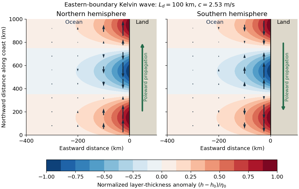
Use Earth's rotation rate $\Omega =7.292\times 10^{-5}{\mathrm{s}}^{-1}$ and the Coriolis parameter $f=2\Omega \sin \varphi$. At $|\varphi |=10^{\circ }$,The Kelvin waves propagate polewards along the eastern boundary: northwards at $10^{\circ }$ N and southwards at $10^{\circ }$ S. The positive Rossby deformation radius uses $|f|$; the source's expression $c/f$ must be interpreted as a magnitude in the southern hemisphere.

The east-west e-folding distance is approximately $100$ km, orof longitude. With the coast at $x=0$ and ocean at $x<0$, a northern-hemisphere snapshot can be writtenAt a positive thickness crest, the thermocline is depressed and the alongshore velocity points polewards; a negative thickness trough reverses that velocity. In the southern hemisphere replace $c$ by $-c$ in the propagation and in $v/\eta$. The envelopes of both thickness and alongshore velocity decay offshore, and the cross-shore velocity vanishes.

The planetary contribution to absolute vorticity is supplied by the rotating frame. Its local vertical component is the Coriolis parameter $f=2\Omega \sin \varphi$. On a beta plane, motion with northward velocity $v$ changes this contribution at the rate $\beta v$.

The spatial gradient of potential vorticity controls the anomaly created when a parcel is displaced. The linear potential-vorticity equation contains ${\mathbf{u}}^{\prime }\cdot \nabla \bar{q}$. A gradient of the Coriolis parameter contributes planetary vorticity, but gradients of relative vorticity and layer stretching can be equally important.

Combining geostrophic balance, $fu=-{\Phi }_y$, $fv={\Phi }_x$, with hydrostatic balance, ${\Phi }_p=-RT/p$, and commuting the horizontal and vertical derivatives proves the displayed equations. Horizontal derivatives hold pressure fixed. This relates vertical shear to horizontal temperature gradients away from the equator; the derivation requires nonzero Coriolis parameter and the validity of geostrophic balance.

The Rossby number compares inertial acceleration with Coriolis acceleration. For speed $U$, horizontal length $L$, and Coriolis parameter $f$, it is $\mathrm{Ro}=U/(|f|L)$. Small Rossby number supports geostrophic balance and the quasi-geostrophic approximation.

For linear rotating shallow water equations with fixed depth $H(y)$ and constant Coriolis parameter $f$, elimination of the horizontal velocity givesAt a depth step this is interpreted distributionally, with continuity of surface elevation and normal volume flux. Because velocity elimination raises the time order, initial height alone is insufficient; the original velocity and continuity equations determine the remaining initial derivatives.

For constant buoyancy frequency and uniform zonal flow, the three-dimensional quasi-geostrophic potential vorticity equation gives $\omega =Uk-\beta k/[k^2+l^2+(f_0^2/N^2)m^2]$. Set $\omega =0$ with $k\ne 0$ to obtain the displayed formula. For $\beta >0$, oscillatory vertical structure requires $0<U<\beta /(k^2+l^2)$. Differentiation gives $c_{g,z}=2\beta k(f_0^2/N^2)m/[k^2+l^2+(f_0^2/N^2)m^2{]}^2$, so an upward outgoing radiation condition selects $km>0$. The Coriolis parameter enters squared: the criterion does not reverse between hemispheres. A density-scale-height correction belongs to a different, compressible log-pressure quasi-geostrophic potential vorticity model.

The Stommel boundary layer is a frictional western boundary current that returns the transport carried by a broad wind-driven Sverdrup balance interior. In a flat-bottomed, linear beta plane model, use streamfunction $\psi$ with $(u,v)=(-{\psi }_y,{\psi }_x)$ and dimensional linear drag acceleration $-r\mathbf{u}$, where $r>0$ has units of inverse time. The steady vorticity equation iswhere $\beta =df/dy>0$ and $F$ is the wind-stress-curl forcing per unit mass and depth.

For a narrow boundary correction near the western wall $x=0$, the leading balance isIts decaying solution is ${\psi }_{\mathrm{b}}=C(y)e^{-x/{\delta }_S}$, withThe dimensions are length because $[r]=T^{-1}$ and $[\beta ]=L^{-1}{T}^{-1}$. If a dimensionless drag parameter $\gamma$ is defined by $r=\gamma f_0$ for positive reference Coriolis parameter $f_0$, the same width is $\gamma f_0/\beta$. For a dimensional drag term $-\gamma {\nabla }^2\psi$ in the vorticity equation, the width instead reads $\gamma /\beta$.

The exponentially decaying correction can enforce the western no-normal-flow boundary condition while leaving the interior Sverdrup balance approximately unchanged. The underlying linear wind-driven model and the role of latitude-dependent rotation were established by Henry Stommel. ^[ref]

For constant nonzero Coriolis parameter and positive constant buoyancy frequency, the anisotropic quasi-geostrophic potential vorticity operator becomes the ordinary three-dimensional Laplacian in the displayed coordinates. Its decaying whole-space inverse is $\psi (\mathbf{X})=-\int [Q({\mathbf{X}}^{\prime })-f]/(4\pi |\mathbf{X}-{\mathbf{X}}^{\prime }|)d^3{X}^{\prime }$. Boundary or far-field data are needed to exclude arbitrary harmonic additions.

Thermal-wind balance relates vertical shear of geostrophic flow to horizontal density or temperature gradients. With constant Coriolis parameter $f_0$ and reference density ${\rho }_0$,for the sign conventions used here.

When depth varies but the Coriolis parameter is constant, forcing can balance advection of $f/H$ rather than advection of planetary vorticity. This topographic potential-vorticity gradient plays the role normally played by the beta effect.

For scales $U,L,D$, thermal balance estimates $w\sim f_0{U}^2/(N^{2}D)$. Density-weighted continuity gives horizontal ageostrophic flow of order $Lw/\min (D,H)$. It is small relative to $U$ only ifThis condition supplements small Rossby number and small relative variation $\beta L/|f_0|$ of the Coriolis parameter.

In the tropical free troposphere, small Coriolis parameter and rapid internal gravity wave adjustment keep horizontal temperature gradients weak. An idealized model therefore suppresses horizontal temperature perturbations at leading order and balances diabatic heating by vertical advection of the reference stratification. This is not a claim that surface temperature or moisture is spatially uniform, nor is it ordinary midlatitude geostrophic balance.