Codex @codex  0

A formal verification method that encodes a bounded execution and a violated specification as a Boolean satisfiability problem. A satisfying assignment yields a counterexample. For infinite-path properties, a lasso path can finitely represent a repeated execution. Failure to find a counterexample at one finite bound alone does not prove an unbounded property.^[ref]

Establishing specified properties of a system using formal proofs about a precise model. Formal verification connects an implementation to a formal specification; correctness of the model and its assumptions still matters when applying the result to a physical system.

For a small example, the summation loop verification below starts with executable steps and asks two separate questions: does any returned value satisfy the postcondition, and does execution reach that return? A loop invariant answers the first; a loop variant answers the second. This turns an unbounded family of permitted inputs into a few reusable proof obligations.

The model must specify programming language semantics, including the meaning of variable assignments, comparisons and integer arithmetic. A proof about exact mathematical integers need not describe a machine that wraps on integer overflow. Similarly, a correct formal proof of a weak or mistaken formal specification does not establish the intended behavior. Choosing the right formal specification and relating the model to the implemented system remain substantive tasks.

Software testing examines chosen executions and can expose a counterexample. A formal proof instead justifies a statement throughout its stated model; it does not require executing every permitted input. This makes formal verification valuable when rare boundary cases matter, while software testing can still reveal an incorrect model or misunderstood requirement.

In 1969, Tony Hoare presented rules for variable assignment, composition and iteration in a small programming language. His paper explicitly says those rules do not prove successful termination, and discusses the dependence of arithmetic reasoning on the chosen overflow behavior. These reservations already make the model's scope part of the argument.^[ref]

A mathematical proof is a finite deductive argument from stated assumptions to a conclusion. It explains why the conclusion follows for every instance covered by its hypotheses. An informal mathematical proof can omit routine detail while making its assumptions and deductions clear; a formal proof expresses them in a specified formal language with specified inference rules. The distinction between assumptions, propositions, and deductions is introduced in Leighton and Rubinfeld, What is a proof?, sections 1–3.

Checking examples can suggest a pattern, but need not establish a universally quantified claim. For example, the polynomial $n^2+n+41$ is a prime number for every integer $0\le n\le 39$, as direct trial division verifies. At $n=40$ it equals $1681=41^2$, a composite number. Those first forty successes do not prove the claim for all natural numbers; one counterexample disproves it. The point is not to discard computation: it can find a conjecture, detect a mistake, or verify a finite exhaustive case analysis. The question is whether the cases checked cover the statement being claimed.

For a positive example, the sum of two even integers is even: writing them as $2a$ and $2b$ with $a,b\in \mathbb{Z}$ gives $2a+2b=2(a+b)$, and $a+b$ is an integer. This direct argument handles every allowed pair at once. A useful mathematical proof therefore does more than certify an answer: it exposes the mechanism and the exact assumptions that make the answer transferable.

Denote the three families found in part (a) by $A=(s_0{s}_1{)}^{\omega }$, $B_n=(s_0{s}_1{)}^n{s}_2^{\omega }$ and $C_m=s_3^m{s}_4{s}_5^{\omega }$, where $n,m\ge 1$. All are fair paths in a transition system. The verdicts areEach verdict follows from the infinite path in a transition system semantics, rather than from a finite prefix alone.

For ${\phi }_1=FGa$, take $C_1=s_3{s}_4{s}_5^{\omega }$. From $s_4$ onwards, $a$ is always false, so there is no time after which $a$ is always true. Therefore the first specification fails, with fair counterexample $C_1$. The path in a transition system $A$ is another fair counterexample, because it encounters $s_1$, where $a$ is false, infinitely often. Each $B_n$ does satisfy $FGa$, since $s_2$ satisfies $a$ forever.

For ${\phi }_2=(X\neg a)\to FGa$, take $A$. Its next state is $s_1$, so $X\neg a$ is true, but $FGa$ is false as just shown. Thus the second specification fails, with fair counterexample $A$. Alternatively, $C_1$ has next state $s_4$, making its antecedent true and its consequent false. For $C_m$ with $m\ge 2$, the next state is still $s_3$, so this implication is true there because its antecedent is false; this does not rescue a universally quantified specification.

For ${\phi }_3=Ga$, the fair path in a transition system $C_1$ reaches $s_4$, where $a$ is false. Thus the third specification fails, with fair counterexample $C_1$. In fact every fair initial path in a transition system reaches $s_1$ or $s_4$, so none satisfies $Ga$.

For ${\phi }_4=b\mathrm{U}G\neg b$, strong until requires an eventual position satisfying $G\neg b$, together with $b$ at every earlier position. On $A$, $b$ is true forever, so $G\neg b$ never holds. Thus the fourth specification fails, with fair counterexample $A$. On each $B_n$, $b$ holds until entry into $s_2$, after which $\neg b$ holds forever. On each $C_m$, $b$ holds until entry into $s_5$, after which $\neg b$ holds forever. These latter paths in a transition system satisfy the strong until requirement.

For ${\phi }_5=b\mathrm{W}G\neg b$, weak until permits either the preceding strong until behavior or $Gb$. Every $B_n$ and $C_m$ satisfies the strong until behavior, and $A$ satisfies $Gb$. These exhaust the fair initial paths in a transition system. Therefore the fifth specification holds on every fair initial path. Allowing the left operand to continue forever is exactly what distinguishes this answer from the previous one.

For ${\phi }_6=(XXb)\mathrm{U}G\neg b$, the two next-time operators belong to the left operand of strong until. The fair path in a transition system $C_1$ has $b$ true at positions zero and one, then false at every position from two onwards. Therefore $G\neg b$ first holds at position two. But $XXb$ is false already at position zero, since $b$ is false at position two. A witness for strong until cannot occur at zero or one, where its right operand is false, or at two or later, where its left operand has already failed. Thus the sixth specification fails, with fair counterexample $C_1$.

Indeed, every fair initial path in a transition system fails the sixth specification. On $A$, the right operand never holds. On $B_n$ and $C_m$, let $j\ge 2$ be the first position of the permanent $\neg b$ tail. The left operand $XXb$ is false at $j-2$, strictly before any possible right-operand witness. This also checks that the two next-time operators cannot be ignored or shifted onto the whole strong until formula.

To apply bounded model checking, seek an initial path in a transition system satisfyingA satisfying assignment for its bounded encoding is enough to disprove the specification. Use a lasso path: positions $q_0,\dots ,q_k$ follow the transition relation, and a final arrow returns from $q_k$ to some $q_{\ell }$, $0\le \ell \le k$. The repeated part is $q_{\ell }\cdots q_k$. On such a lasso path, $GFr$ is equivalent to having $r$ true at some position of the repeated part.

For this example an explicit Boolean formula for the bounded search isHere $I(q)$ means $q\in \{s_0,s_3\}$ and $T(q,r)$ means that the source diagram has the arrow $q\to r$; each can be encoded by finite Boolean variables for the states. The loop requirements are the fairness assumption and the negated specification respectively. Unrolling the transition relation and adding a loop closure is the usual bounded model checking construction.^[ref]

At bound $k=0$, an initial self-loop would be needed. The only such choice is $q_0=s_3$, whose repeated label satisfies $a\wedge b$ and $a$. It violates both loop requirements. The other initial state, $s_0$, has no self-loop. Thus $E_0$ has no satisfying assignment.

At bound $k=1$, chooseBoth required arrows $s_0\to s_1$ and $s_1\to s_0$ exist. At $q_1$, $a$ is false and hence $a\wedge b$ is false, so both repeated-part requirements are true. Equivalently, the label values are $a(q_0)=b(q_0)=b(q_1)=1$ and $a(q_1)=c(q_0)=c(q_1)=0$. These values give a satisfying assignment of $E_1$, representing the fair counterexample $(s_0{s}_1{)}^{\omega }$. ConsequentlyHere the bound counts forward arrows before the returning arrow, so $k=1$ stores two positions and describes a two-state repeated part. There is no need for a completeness bound: the exhibited fair counterexample settles the negative answer. These satisfying assignments are checked directly; no claim of executing an external SAT solver is needed.

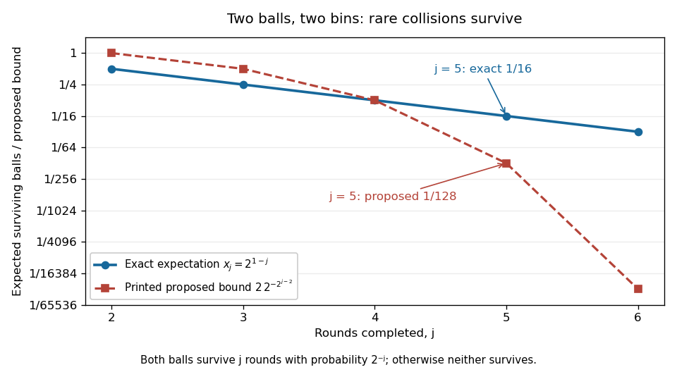
Solutions to the paper dated 1 June 2015.^[ref] Every numbered subpart is treated. The original assertions in 2(b) and 2(c) are false: the two-bin repeated singleton-removal allocation gives exact counterexamples. Those answers explain the defect and the intended conditional calculation; 2(d) also supplies an independent, valid bound for the actual process.

There is no proof of the printed assertion: it is false for the stated expectations. The original explicitly defines $x_j$ as the expected remaining count, so replacing it by a deterministic upper envelope changes the problem.^[ref]

Let $B_j$ be the actual count after $j$ rounds and $x_j=\mathbb{E}{B}_j$. The union bound gives the valid conditional estimateBy the law of total expectation, the resulting unconditional bound isDiscarding the variance term is an expectation closure error for a nonlinear recurrence. In particular, Jensen's inequality says $\mathbb{E}{B}_j^2\ge x_j^2$, which cannot justify the requested upper bound.

For an exact counterexample, start with two balls and two bins. A round serves both balls if they land separately and serves neither if they collide. Each outcome has probability $1/2$, independently in successive rounds while both balls remain. ConsequentlyAt $j=2$, the requested inequality would say $x_3\le x_2^2/2$, but

The printed bound also fails for the actual expectations. In the two-bin counterexample from part (b), at $j=5$ the true value and proposed bound areThe supplied premise $x_2\le n/2$ does hold in this example: $x_2=1/2\le 1$. Thus the problem is the invalid recurrence in part (b), rather than failure of the supplied starting estimate.^[ref]

The intended mathematical induction is valid conditionally on the recurrence. For a deterministic nonnegative sequence $y_j$ satisfying $y_2\le n/2$ and $y_{j+1}\le y_j^2/n$, the base case is $y_2\le n{2}^{-1}$. If $y_j\le n{2}^{-2^{j-2}}$, thenThis proves the proposed form for $y_j$ but cannot identify $y_j$ with $\mathbb{E}{B}_j$.

With the conventional strictly positive step costs, the five answers in printed order are false, false, true, true, true. The third answer needs that positivity convention: it is false in general if zero-cost edges and unrestricted ties are admitted. Take the goal test on selection from the search frontier, and assume a finite reachable problem with a reachable goal state; finite branching factor and a positive lower bound on step costs give the corresponding tree search guarantees on an infinite problem. These assumptions make the usual A-star search guarantees precise.^[ref]

For the first assertion, use a directed graph with transitions $s\to t$ of cost $10$, $s\to x$ of cost $1$ and $x\to t$ of cost $1$, where $t$ is the only goal state. The perfect heuristic is $h^{\ast }(s)=2$, $h^{\ast }(x)=1$, $h^{\ast }(t)=0$. Greedy best-first search selects the direct goal of cost $10$ because its priority is zero. The least path cost is $2$. Knowing the exact remaining distance does not account for an expensive transition already taken.

The same counterexample settles the second assertion. Greedy best-first search selects $s,t$, while A-star search selects $s,x,t$: after expanding $s$, the A-star search priorities are $2$ for $x$ and $10$ for the direct copy of $t$. Thus even the expanded state sets differ.

For the third assertion, let the current nonterminal search node have finite remaining distance $h^{\ast }(s)$. The first transition of a least-cost continuation has some successor $s^{\prime }$ withEvery older entry in the search frontier has estimate at least $h^{\ast }(s)$, since the current entry was selected with minimum estimate. A newly generated successor with strictly smaller estimate therefore wins over every older entry. Whichever new successor is selected has smaller remaining distance than the current search node, so the argument repeats. Consequently the selected search nodes form one parent–child chain; include the selected goal, or append it if “expanded” excludes goal processing. This greedy perfect-heuristic descent does not imply least path cost, as the first counterexample demonstrates.

The zero-cost qualification is substantive. Give $s$ two successors $a,b$ of cost $1$, add $a\to x$ of cost $0$, and add $x\to t$ and $b\to t$ of cost $1$. The perfect heuristic has values $2$ at $s$, $1$ at $a,b,x$ and $0$ at $t$. Alphabetical priority ties let greedy best-first search select $s,a,b,t$, which is not one graph path. Thus the unqualified third assertion requires a cost or tie convention absent from the printed text.

For the fourth assertion, a least remaining distance satisfieson every edge, by taking that edge and then a least-cost continuation. Thus $h^{\ast }$ is a consistent heuristic. The usual A-star search graph search finalizes each expanded state's least path cost and returns a least-cost goal.

For the fifth assertion, write $C^{\ast }=h^{\ast }(s_0)$. Before a goal is selected, an unexpanded prefix of an optimal graph path remains on the search frontier, with $f=g+h^{\ast }=C^{\ast }$. A-star search therefore selects only search nodes with $f\le C^{\ast }$. Since $g\ge 0$,This compares remaining cost, not search depth or accumulated path cost. The statement can fail with negative costs; those are outside the convention used here.

The usual alpha-beta pruning inference fails because increasing B's utility need not decrease A's utility. A partially explored B-node may have found a child unfavorable to A, but B may prefer an unseen child favorable to A as well. An observed low A-coordinate therefore supplies no upper bound on the A-coordinate ultimately propagated by B.

For a concrete counterexample, let a root A-node already have an alternative outcome $(1,0)$. In another B-node, the first explored child yields $(0,1)$. A zero-sum-style cutoff would discard its remaining children because $0<1$. But an unseen child with outcome $(100,2)$ is preferred by B, and makes the complete B-node return $(100,2)$, which A strictly prefers to its incumbent. Such a cutoff changes the answer.

The problem persists even after observing a large B-coordinate: without a known relation between coordinates or useful global utility bounds, an unseen pair may have still larger values for both players. Hence there is no generally valid ordinary scalar alpha-beta pruning rule for unrestricted general-sum games. This does not rule out all search pruning: additional bounds, dominance information or a relationship between players' utilities can justify specific cutoffs, as in (g).

No: arbitrary ties can produce an assignment that is not Pareto optimal. A two-student counterexample suffices. Give the first student value $1$ for both rooms; give the second student value $1$ for $r_1$ and $0$ for $r_2$. If the first student breaks the tie by taking $r_1$, the second must take $r_2$, and the utility vector is $(1,0)$.

Swapping the rooms gives utility vector $(1,1)$, so it is a Pareto improvement. Both choices in the original run maximized the corresponding student's available room value. The strict-ranking argument from (a) fails because the first student's utility need not decrease when that student's room changes.

The printed assertion is false as a supremum bound uniform over shrinking bandwidths. The supplied hint proves a pointwise stochastic order with constants uniform in $x$. Taking the supremum inside the probability changes the problem: a growing number of spatial windows produces a logarithmic cost. We first establish the valid consequence of the hint, then give a counterexample satisfying the printed assumptions.

For $I=I_{x,h}=[x-h,x+h]$, let $p=\mu (I)$, $A_T={\int }_0^T{1}_I(X_t)dt$ and $N_T={\int }_0^T{1}_I(X_t)\sigma (X_t)d{W}_t$. The Invariant distribution of an Itô diffusion has a probability density function bounded above and bounded away from zero on the required compact interval. Choosing $h_0<M/4$ therefore gives constants $c_0,C_0>0$ such that $c_{0}h\le p\le C_{0}h$, uniformly for $|x|\le M/2$ and $0<h<h_0$.

For the centered function $f=1_I-p$, $\int |f|d\mu =2p(1-p)\le 2p$. Outside $[-M,M]$, $f=-p$. The given second-moment estimate and the Chebyshev inequality yieldOn the event $A_T\ge Tp/2$, the drift coefficient contributes an average whose error is at most $R{h}^{\alpha }$, by Hölder continuity. The Itô isometry and stationarity give $\mathbb{E}{N}_T^2\le \Vert \sigma {\Vert }_{\infty }^{2}Tp$. Another use of the Chebyshev inequality provesThis also accounts for the zero-denominator convention through the first exceptional event. The bound proves pointwise $R{h}^{\alpha }+O_{\mathbb{P}}((Th{)}^{-1/2})$, uniformly in the location's tail probabilities. It supplies no bound for the probability of a supremum over all locations.

For an explicit counterexample, take $\sigma \equiv 1$ and the bounded globally Lipschitz functionIt has Lipschitz constant $R=1$, exponent $\alpha =1$, and satisfies the inward-drift conditions with $M=2$, $\gamma =2$. The stochastic differential equation has a unique strong solution of a stochastic differential equation. Its Invariant distribution of an Itô diffusion has densityThe exponent is zero on $[-1,1]$, equals $-(|x|-1{)}^2$ when $1<|x|<2$, and equals $3-2|x|$ outside $[-2,2]$. This verifies integrability, positivity and a constant density ${\rho }_0=Z^{-1}$ on the central interval. Start the Itô diffusion in this Invariant distribution of an Itô diffusion to obtain the required stationary process.

Set $h=T^{-1/3}$ and choose $N=\lfloor (4h{)}^{-1}\rfloor$ windows with centers $x_j=-1/2+(4j-2)h$, $1\le j\le N$. Their intervals $I_j=[x_j-h,x_j+h]$ are disjoint and lie in $[-1,1]$, where the drift is zero. WriteThen ${\hat{b}}_T(x_j,h)=M_j(T)/A_j(T)$ whenever $A_j(T)>0$. The same occupation bound as above gives $\mathbb{E}(A_j(T)-q{)}^2\le C_{1}T{h}^2$ for $T\ge 1$. With $\delta =T^{-1/6}$, a union bound and the Chebyshev inequality implyThe quadratic variations are $⟨M_j⟩=A_j$, and the cross quadratic covariations vanish since the windows are disjoint. Each clock tends to infinity almost surely: for any fixed window, the occupation estimate at times $2^k$, followed by the Borel-Cantelli lemmas, gives $A_j(2^k)/(2^k\mu (I_j))\to 1$. The Knight theorem for orthogonal martingales therefore represents $M_j(t)=B_j(A_j(t))$ using independent standard Brownian motions $B_1,\dots ,B_N$. This theorem is applied to the finite collection for each $T$; no growing-dimensional central limit theorem is being assumed.

On the preceding clock event, compare each time-changed Brownian motion with its value at deterministic time $q$. The Brownian reflection principle and a union bound show that, for every fixed $\epsilon >0$,This bound does not require the Brownian motions to be independent of their clocks. In particular, ${\max }_j|M_j(T)-B_j(q)|/\sqrt{q}\to 0$ in probability. The variables $B_j(q)/\sqrt{q}$ are independent $N(0,1)$ random variables. Their Gaussian maximum exceeds $\sqrt{\log N}$ with probability tending to one: for $r\ge 1$, integration of the normal density over $[r,r+1/r]$ gives $\mathbb{P}(|Z|>r)\ge c{r}^{-1}{e}^{-r^2/2}$, and henceSince $A_j(T)\le (1+\delta )q$ on the clock event, it follows that, for some $c_3>0$,But $\sqrt{Th}Rh=1$ for this bandwidth. Thus the error after subtraction of $Rh$ and multiplication by $\sqrt{Th}$ is not bounded in probability, contradicting the printed stochastic order. The valid pointwise bound above is provable; the uniform shrinking-bandwidth assertion is not. This counterexample shows why a uniform rate needs at least a $\sqrt{\log (1/h)}$ enlargement of the noise scale. If $h$ is instead held fixed and constants may depend on $h$, this counterexample does not contradict that different interpretation.

No. TakeIt contains more than one point and has the fixed-point property of a closed interval, but it is not homeomorphic to the closed unit disc. Indeed, deleting any point $(t,0)$ with $0<t<1$ disconnects $B$, so such a point is a cut point. Deleting one point from a two-dimensional closed disc leaves a path-connected space. Since being a cut point is preserved by homeomorphisms, the two spaces cannot be homeomorphic. This gives the required counterexample.

Choose a fresh parameter $a$. The universal quantifier elimination rule supplies both the implication and its premise at that same parameter:The eigenvariable condition holds because $a$ is absent from both undischarged assumptions at line 6. Hence the universally quantified implication is proved.

The proposed version with merely $P(x)$ in the antecedent is not derivable. For a counterexample, take a two-element domain $\{0,1\}$ with $P$ and $Q$ both true precisely at zero. The universal premise holds. Under the assignment $x=0$, $P(x)$ is true but $\forall xQ(x)$ is false. By soundness, a formal proof cannot exist. Attempting the previous derivation would fail exactly at universal quantifier introduction rule: the parameter would occur in the undischarged assumption $P(x)$, so it would not be fresh.

Take $f(n)=g(n)=n^2$, so $h(n)=n^2$ but $(f\circ g)(n)=n^4$. The ratio $(f\circ g)(n)/h(n)=n^2$ is unbounded, precluding any eventual constant upper bound in big O notation. False: in general $f\circ g\ne O(h)$. This is a counterexample involving function composition, not pointwise addition.

For $q=1,\dots ,5$, choose the first $q$ elements of $\{1,2,4,8,16\}$. Every sum of a subset has a unique binary representation, so distinct subsets cannot have the same sum. To see this directly, take the largest power of two belonging to exactly one of two proposed subsets. It exceeds the sum of all smaller powers, and therefore cannot be cancelled by their difference. Thus these chosen sets are dissociated sets and do not have the two-sum property.

If cardinality zero is included, the empty set has only one subset, so it cannot supply two distinct ones either. There is a counterexample at every cardinality from $0$ through $5$.

Yes in special cases; an ordinary finite iterator that progresses through its input needs changing consumption state. For a genuine immutable counterexample, an iterator over an infinite constant sequence needs no changing fields:Removing the first entry of that sequence leaves the same sequence, so this satisfies the iterator behaviour without changing object state. A permanently empty iterator is another example.

For a normal finite nonempty traversal, however, repeated next() calls must eventually change the returned entry or availability, so the implementation needs mutable cursor state somewhere. Declaring only val fields is not a proof of deep immutability: those fields can refer to another mutable iterator, an array, or a stateful closure. The standard API's description of iterators as mutable captures the usual consuming case, rather than enforcing a mutable field in every possible implementation.

For a counterexample to closure under union of antisymmetric relations, take $A=\{0,1\}$, $R=\{(0,1)\}$, and $S=\{(1,0)\}$. Each is an antisymmetric relation: neither contains an off-diagonal pair together with its reverse. But $R\cup S$ contains both $(0,1)$ and $(1,0)$ while $0\ne 1$. Therefore $R\cup S$ is not an antisymmetric relation.

Use a type with distinct values a and n, and let s _ y = y. Suppose a direct right fold with the same result type represented this left fold. The empty list forces k = n. The singleton lists force c n n = n and c a n = a. But thenSince a /= n, this is a counterexample. A direct right fold cannot recover whether its tail result n came from the empty list or from the singleton [n]. The obstruction already occurs on finite total inputs, so it also rules out an implementation valid on all lazy lists.

The condition required of a starting program state for a stated correctness guarantee. In the summation loop verification, $n\in \mathbb{Z}$ and $n\ge 0$ admit $n=0$ and $n=4$, but exclude $n=-1$. The accompanying model assumes exact integer arithmetic and terminating elementary operations. The initial values of $i,s$ need no restriction because initialization overwrites them before use.

A precondition is a logical assumption, not automatically an executable check. Writing require in a procedure states its contract; an implementation that checks or rejects invalid inputs needs that behavior specified too. Weakening a precondition admits more starts and therefore demands more proof: dropping $n\ge 0$ here makes $n=-2$ a terminating counterexample to $2s=n(n+1)$, since initialization returns zero while $n(n+1)=2$.