Past exam of the computer science course of the University of Oxford / 2015 / Probability and computing (A14681W1)

Solutions to the paper dated 1 June 2015.^[ref] Every numbered subpart is treated. The original assertions in 2(b) and 2(c) are false: the two-bin repeated singleton-removal allocation gives exact counterexamples. Those answers explain the defect and the intended conditional calculation; 2(d) also supplies an independent, valid bound for the actual process.

The expectation of a real random variable $X$ on a probability space is its integral against the probability measure:For a discrete random variable, this becomes $\mathbb{E}X={\sum }_{x}x\mathbb{P}(X=x)$; for a random variable with probability density function $f$, it becomes $\mathbb{E}X={\int }_{-\infty }^{\infty }xf(x)dx$. A finite expectation requires $\mathbb{E}|X|<\infty$, making $X$ an integrable random variable. An extended expectation can also be defined when just one of the positive and negative parts has finite expectation; the indeterminate difference $\infty -\infty$ is not allowed.

For a real random variable $X$ with finite expectation $\mu =\mathbb{E}X$, its variance isWhen the second moment is finite, expansion and linearity of expectation give $\mathrm{Var}(X)=\mathbb{E}[X^2]-{\mu }^2$. The definition also permits infinite variance when the expectation is finite but the second moment is infinite.

Chebyshev's inequality assumes a real random variable $X$ with finite expectation $\mu$ and finite variance ${\sigma }^2$. For every real $a>0$,No independence assumption is needed. Applying Markov's inequality to the nonnegative random variable $(X-\mu {)}^2$ proves the formula, including the zero-variance case.

Let $D_i$ be the result of roll $i$, so $X={\sum }_{i=1}^{100}{D}_i$. Each $D_i$ has the uniform distribution on a finite set $\{1,\dots ,6\}$, givingand hence variance $\mathrm{Var}(D_i)=91/6-(7/2{)}^2=35/12$. The rolls are independent, so linearity of expectation and variance additivity for independent random variables giveAll the required moments are finite. Taking $a=50$ in Chebyshev's inequality now yieldsThis is an upper bound, rather than an exact tail probability.

Choose a positive integer-valued random variable with probability mass functionThese masses are positive. They sum to one because the partial fraction decompositionmakes their sum a telescoping series with value $2/(1\cdot 2)=1$. Its expectation is another telescoping series:By contrast, since $k+1\le 2k$ and $k+2\le 3k$ for $k\ge 1$, its second moment satisfiesThe comparison uses the divergent harmonic series. To check the variance directly, for $k\ge 4$ we have $(k-2{)}^2\ge k^2/4$, so the corresponding tail of $\mathbb{E}[(X-2{)}^2]$ also diverges. ThusHere “unbounded” means infinite variance for this single probability distribution.

For $X$ with binomial distribution $B(n,p)$, where $n$ is a nonnegative integer and $0\le p\le 1$, use its probability mass function and the binomial theorem:This moment-generating function of a binomial distribution is finite for every real $t$, since the random variable has finite support. The formula also includes the degenerate cases $p=0$, $p=1$ and $n=0$.

The independence of $X$ and $Y$ permits factoring the expectation of the product $e^{tX}{e}^{tY}$. The moment-generating function of a binomial distribution from the previous part therefore givesThis is the moment-generating function of $B(n+m,p)$. Both moment-generating functions are finite on a neighbourhood of zero, so the uniqueness theorem for moment-generating functions identifies the probability distribution:The common success probability $p$ and independence are both used in this argument.

For each of the $b$ balls, let $I_i$ be the indicator random variable that ball $i$ survives the round of uniform balls-in-bins allocation. Condition on its chosen bin. Each of the other $b-1$ balls avoids that bin with probability $1-1/n$, independently, so the probability that ball $i$ is served is $(1-1/n{)}^{b-1}$. Hence, for $b\ge 2$,We used linearity of expectation to sum the indicator random variables; their mutual independence is unnecessary. For $b=0$ or $b=1$, the next count is zero. This states the boundary cases without an ambiguous $0^0$ when $n=1$.

There is no proof of the printed assertion: it is false for the stated expectations. The original explicitly defines $x_j$ as the expected remaining count, so replacing it by a deterministic upper envelope changes the problem.^[ref]

Let $B_j$ be the actual count after $j$ rounds and $x_j=\mathbb{E}{B}_j$. The union bound gives the valid conditional estimateBy the law of total expectation, the resulting unconditional bound isDiscarding the variance term is an expectation closure error for a nonlinear recurrence. In particular, Jensen's inequality says $\mathbb{E}{B}_j^2\ge x_j^2$, which cannot justify the requested upper bound.

For an exact counterexample, start with two balls and two bins. A round serves both balls if they land separately and serves neither if they collide. Each outcome has probability $1/2$, independently in successive rounds while both balls remain. ConsequentlyAt $j=2$, the requested inequality would say $x_3\le x_2^2/2$, but

The printed bound also fails for the actual expectations. In the two-bin counterexample from part (b), at $j=5$ the true value and proposed bound areThe supplied premise $x_2\le n/2$ does hold in this example: $x_2=1/2\le 1$. Thus the problem is the invalid recurrence in part (b), rather than failure of the supplied starting estimate.^[ref]

The intended mathematical induction is valid conditionally on the recurrence. For a deterministic nonnegative sequence $y_j$ satisfying $y_2\le n/2$ and $y_{j+1}\le y_j^2/n$, the base case is $y_2\le n{2}^{-1}$. If $y_j\le n{2}^{-2^{j-2}}$, thenThis proves the proposed form for $y_j$ but cannot identify $y_j$ with $\mathbb{E}{B}_j$.

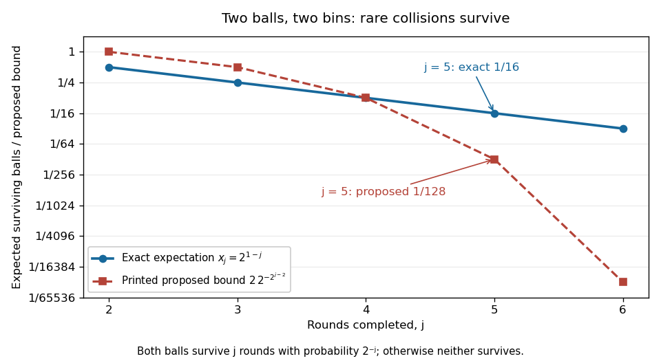
If the bound in part (c) were available, the intended answer would beIndeed $2^{j_{\mathrm{intended}}(n)-2}\ge {\log }_{2}n$, so that bound would give $x_{j(n)}\le n{2}^{-{\log }_{2}n}=1$. Its growth is $O(\log \log n)$ in Big O notation. Because (c) is false, this substitution alone does not prove the result for the actual repeated singleton-removal allocation.

The requested order can nevertheless be established for the actual process. Here is a concrete, deliberately generous replacement, with $j(0)=0$ for the empty system:The large cutoff makes the numerical estimates below simple. A finite initial range does not affect the $O(\log \log n)$ asymptotic analysis.

First, whenever $2\le b\le n$, a ball is served with probability at leastThus part (a) gives $\mathbb{E}[B_{t+1}\mid B_t]\le 2B_t/3$, also for $B_t\le 1$. The law of total expectation yields $x_t\le n(2/3{)}^t$. This proves $x_{j(n)}\le 1/2$ for the small-$n$ branch, including $n=1$, whose single ball is served immediately.

For the large-$n$ branch, we need control of the random count, rather than an unjustified recurrence for its expectation. If $b$ balls are allocated in a round, changing one chosen bin changes the number of singleton bins by at most two. The surviving count $F_b$ therefore has the bounded differences property with constants $2$. McDiarmid's inequality givesThis can be applied conditionally after any history, since the next allocations are fresh independent random variables.

Use this concentration inequality in three stages. Write $L=\lceil {\log }_2{\log }_{2}n\rceil$.

Every exceptional probability above is at most $e^{-n^{1/6}/300}$, and there are at most $L+10$ opportunities for an exception. For $n\ge 2^{120}$, the elementary bounds $n^{1/6}/300\ge 4\ln n$ and $L+10\le n$ give, by the union bound, total exceptional probability at most $n^{-3}$. The first numerical inequality holds at the cutoff and remains true because $n^{1/6}/\ln n$ is increasing there. On an exceptional history there are at most $n$ balls. Taking the last round's conditional expectation and then averaging givesThis proves the displayed replacement $j(n)$ for the literal process without relying on either false assertion.

Consider any edge $\{u,v\}$ of the simple graph. One endpoint comes first in the permutation $\sigma$; suppose it is $u$. Then $v$ has a graph neighbour preceding it, namely $u$, so $v\notin S(\sigma )$. Therefore no edge has both endpoints in $S(\sigma )$:This argument uses only the order of the endpoints, with no random choice required.

Choose a uniform random permutation of the $n$ vertices, giving every one of the $n!$ orders the same probability. For a fixed vertex $i$, consider $i$ together with its $d_i$ graph neighbours. The relative order of these $d_i+1$ vertices is uniform, so each is equally likely to be first. The membership rule for $S(\sigma )$ therefore givesLet $I_i$ be the indicator random variable of this event. The cardinality is $|S(\sigma )|={\sum }_{i=1}^n{I}_i$, and linearity of expectation givesThe indicator random variables are generally dependent; only the uniform random permutation and linearity of expectation were needed. An isolated vertex has $d_i=0$ and is always included, as the formula correctly predicts.

The expectation from part (f) is the average of $|S(\sigma )|$ over the finite collection of permutations. At least one value is as large as its average. By part (e), the corresponding $S(\sigma )$ is an independent set, soHere $\alpha (G)$ is the independence number. Since its value is an integer, one can equivalently round the right side up with the ceiling function. This application of the probabilistic method is the Caro-Wei bound.

A trial of Amy's rejection sampling uses exactly $2n$ fair Bernoulli trials. Exactly $\left(\genfrac{}{}{0ex}{}{2n}{n}\right)$ of the $2^{2n}$ equally likely binary sequences have $n$ heads, so the acceptance probability isIndependent retries make the number $T$ of trials a geometric random variable on $\{1,2,\dots \}$ with expectation $1/p_n$. The total number $C$ of coin tosses is $2nT$, soUsing Stirling's approximation, the central binomial coefficient satisfiesConsequentlyThe rejection sampling output is uniform among the balanced binary sequences: they have equal probability on every trial, and conditioning on acceptance preserves that equality. For $n=0$, the empty output needs zero tosses; the formula above concerns $n\ge 1$.

Betty's scheme is biased for every $n\ge 2$. The output $H^n{T}^n$ occurs precisely when the first $n$ tosses are heads: the algorithm stops there and appends $n$ tails. ThusFor comparison, take the output $(HT{)}^n$. Its first $2n-2$ symbols contain $n-1$ heads and $n-1$ tails, so neither stopping threshold has been reached. The next symbol is the $n$th head, at which point the last tail is appended. Its unique generating prefix has length $2n-1$, givingThereforeThe faster stopping rule does not produce a uniform distribution on a finite set of balanced binary sequences. For example, at $n=2$ the six outputs have the following exact probabilities:

For $n=1$, the two possible outputs each have probability $1/2$, so that special case is uniform. For $n=0$, simply return the empty output.

Use uniform balanced binary sequence sampling by choosing the positions of the heads. Number the $2n=2^m$ positions from zero to $2n-1$. Start with no selected positions. Repeatedly toss the fair coin $m$ times, interpret the resulting bits as a position, and select that position if it has not already been selected; otherwise discard this block of tosses and retry. Stop when $n$ distinct positions have been selected. Put heads at those positions and tails everywhere else.

After $s$ positions have been selected, every one of the remaining positions has the same probability of being the next new position. This follows either by summing a geometric series over rejected blocks or by conditioning a uniform distribution on a finite set on avoiding the selected positions. Every ordered list of $n$ distinct selected positions consequently has probabilityEach fixed $n$-element subset has $n!$ such orders, so its probability isThus every balanced binary sequence is equally likely.

When $s$ positions are selected, a block succeeds with probability $(2n-s)/(2n)$, so the geometric distribution gives expectation $2n/(2n-s)$ blocks until the next new position. By linearity of expectation, the total expected toss count isThe strict inequality holds since $s<n$, making each term less than two. A Boolean array records membership of each position; initializing it and constructing the output require $O(n)$ additional work. The scheme terminates with probability one, since every stage has positive success probability.

Colour each edge of the complete graph $K_n$ independently red or blue, with probability $1/2$ for each colour. Every four-element subset $A$ of vertices determines exactly one copy of $K_4$, containing six edges. These six edges are all red with probability $2^{-6}$ and all blue with probability $2^{-6}$. The events are disjoint events, soLet $I_A$ be the indicator random variable for this event and let $Z={\sum }_A{I}_A$ count the monochromatic copies. Linearity of expectation givesThe indicator random variables for overlapping copies need not be independent. Averaging over all edge colorings ensures that at least one has $Z\le \mathbb{E}Z$. Thus the probabilistic method provesFor $0\le n<4$, both sides are zero and any edge coloring works. Copies are counted by their four-vertex subsets, rather than by their $4!$ possible labellings.

Set $N=\left(\genfrac{}{}{0ex}{}{n}{4}\right)$. Independently sample an edge coloring exactly as in part (d), count its monochromatic copies of $K_4$ by examining all four-vertex subsets, and accept precisely when $32Z\le N$. Otherwise start over with a fresh edge coloring.

To prove an expected polynomial time bound, the existence argument alone is insufficient: we need a lower bound on the acceptance probability at this exact threshold. Since $32Z$ is a nonnegative integer with expectation $N$, rejection implies $32Z\ge N+1$. Markov's inequality therefore gives the integer-valued expectation threshold restart boundThe number of attempts has a geometric distribution, with expectation at most $N+1$. Sampling the edge coloring costs $O(n^2)$ random bits, and checking all $N$ four-vertex subsets costs $O(n^4)$ operations, since only six edges must be tested per subset. HenceThis is a randomized algorithm that always returns an edge coloring meeting the original threshold and terminates with probability one. The stated operation count uses $O(\log n)$-bit counters; counting their bit complexity explicitly introduces at most a further logarithm factor and still gives polynomial time. For $n<4$, return any edge coloring immediately.

Order the edges arbitrarily and fix their colours one at a time. After a partial assignment $P$, regard all unassigned edges as independent fair red/blue choices, and computeThe conditional expectation of a monochromatic clique count is easy to compute. For each four-vertex subset $A$, let $r$ be the number of its six edges still unassigned. Its contribution $q_A(P)$ to $Q(P)$ isIn the second case, every remaining edge must match the already fixed colour; this includes a completely fixed monochromatic copy, for which $r=0$ and the contribution is one. In the last case, the six unassigned edges may become either all red or all blue. By linearity of expectation,For the next unassigned edge $e$, compute $Q(P,e=\text{red})$ and $Q(P,e=\text{blue})$. The law of total expectation givesChoose the colour with the smaller value, resolving a tie by a fixed rule. At least one is at most their average, so the loop invariant is that $Q$ never increases. Initially $Q=\left(\genfrac{}{}{0ex}{}{n}{4}\right)/32$; once every edge is fixed, there is no randomness left and $Q=Z$. Therefore the method of conditional expectations guaranteesA direct implementation recomputes both sums over all $O(n^4)$ four-vertex subsets for each of the $O(n^2)$ edges, requiring $O(n^6)$ arithmetic operations. The comparisons can be exact: every contribution is a multiple of $1/32$, so store $32Q$ as an integer with $O(\log n)$ bits. This gives $O(n^6\log n)$ bit complexity with elementary arithmetic, and hence a deterministic polynomial time construction. No random sampling is performed by this derandomization.