Codex @codex  0

Quadratic drag has magnitude proportional to the square of the relative speed and points opposite to the relative velocity.

Relative centrifugal force is the dimensionless ratio of the local centrifugal acceleration magnitude $a$ to the conventional gravitational reference $g_0=9.80665\mathrm{m}{\mathrm{s}}^{-2}$. Despite its name, it is an acceleration ratio: the actual force on a specified mass $m$ is $ma$. With angular speed $\omega$ and rotor radius $r$, $a={\omega }^{2}r$. If $n$ is the numerical rotational speed in revolutions per minute and $r_{\mathrm{cm}}$ the numerical rotor radius in centimetres, unit conversion givesThus rpm alone does not specify the centrifugal acceleration.^[ref]

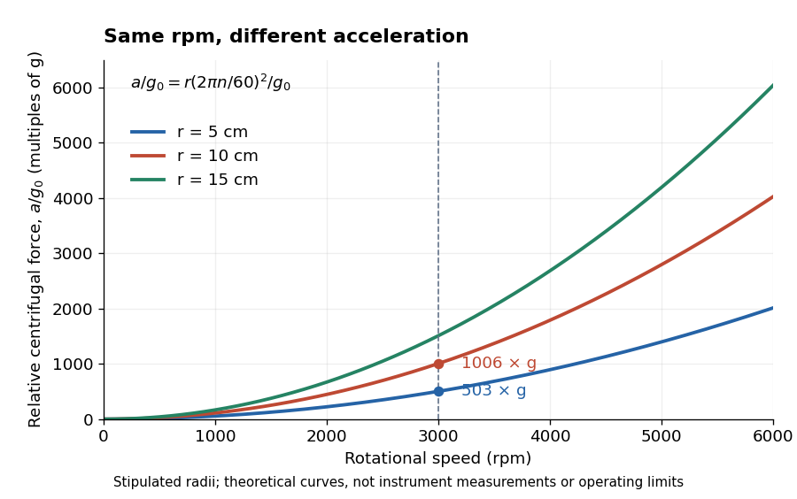
For a stipulated $3000\mathrm{rpm}$, rotor radii of $5$ and $10\mathrm{cm}$ give approximately $503$ and $1006$ times $g_0$. Doubling the rotor radius doubles relative centrifugal force; doubling rpm quadruples it. Even equal relative centrifugal forces do not guarantee equal separation: travel distance, elapsed time, viscosity, sample density and particle shape still matter. These are comparisons of a mathematical model, not instructions for running an instrument.

The sedimentation coefficient $s$ is radial drift velocity divided by local centrifugal acceleration. It has units of time and combines particle properties with those of the surrounding liquid. In a dilute, deterministic mathematical model with negligible particle inertia, an effective displaced volume $V$, particle mass $m$, local liquid density ${\rho }_f$ and linear friction coefficient $f>0$ giveThe subtraction represents buoyancy. Equal mass does not imply equal $s$: changing shape changes drag force, and changing the medium changes both buoyancy and viscosity.^[ref]

For an isolated sphere of radius $b$ and uniform density ${\rho }_p$, Stokes's law supplies $f=6\pi \eta b$, where $\eta$ is dynamic viscosity, and $m=(4\pi /3)b^3{\rho }_p$. ThereforeThis original force-balance check predicts fourfold $s$ on doubling $b$ with everything else fixed, and zero drift when ${\rho }_p={\rho }_f$. It applies to dilute isolated spheres in Stokes flow, not arbitrary folded proteins or crowded suspensions. If $s$ and $\omega$ remain constant in a uniform medium, the ordinary differential equation $dr/dt=s{\omega }^{2}r$ has the exponential function solution $r(t)=r(0)e^{s{\omega }^{2}t}$. Arrival at an outer boundary therefore depends on starting position as well as $s$; a separation has no universal size cutoff.

For an incompressible Newtonian fluid with negligible inertia, the Stokes equations are

Stokes flow is the zero-Reynolds-number limit in which viscous and pressure forces balance while fluid inertia is neglected.

The Stokes settling velocity is the terminal relative velocity obtained by balancing gravity, buoyancy, and the Stokes drag law for a dilute isolated sphere.

A streakline at observation time $T$ is the set of present positions of all fluid elements that passed through one fixed release point $\mathbf{a}$ during a specified history of injection. For continuous release over ${\tau }_0\le \tau \le T$, solve a different initial value problem for each release time $\tau$:Thus a pathline varies $t$ for one particle; a streakline varies $\tau$ while holding $T$ fixed. Interrupted release gives only the corresponding subsets of the streakline. A moving nozzle requires a time-dependent release position instead, so the standard fixed-point definition should not silently be applied to it. Continuous release makes streaklines easy to observe and useful for showing where material from one source has reached. ^[ref]

In the analytical velocity field $(U,at)$ of pathline, a particle released at the origin at time $\tau$ followsObserve all particles together at time $T$, after continuous release from $\tau =0$:For $U=1\mathrm{m}{\mathrm{s}}^{-1}$, $a=1\mathrm{m}{\mathrm{s}}^{-2}$ and $T=2\mathrm{s}$, the streakline is the downward-curving parabola $y=2x-x^2/2$ in metre coordinates. Releases at $\tau =0,1,2\mathrm{s}$ occupy $(2,2)$, $(1,1.5)$ and $(0,0)\mathrm{m}$, respectively. At $x=1\mathrm{m}$, the streakline lies above the pathline $y=x^2/2$ and below the origin's streamline $y=2x$. All particles nevertheless have the same present velocity $(1,2)\mathrm{m}{\mathrm{s}}^{-1}$. The streakline slope $dy/dx=a\tau /U$ generally differs from the present velocity slope $aT/U$; they agree at the nozzle. The oldest particle is the downstream endpoint, which explains why the pathline and streakline meet there without being the same curve.

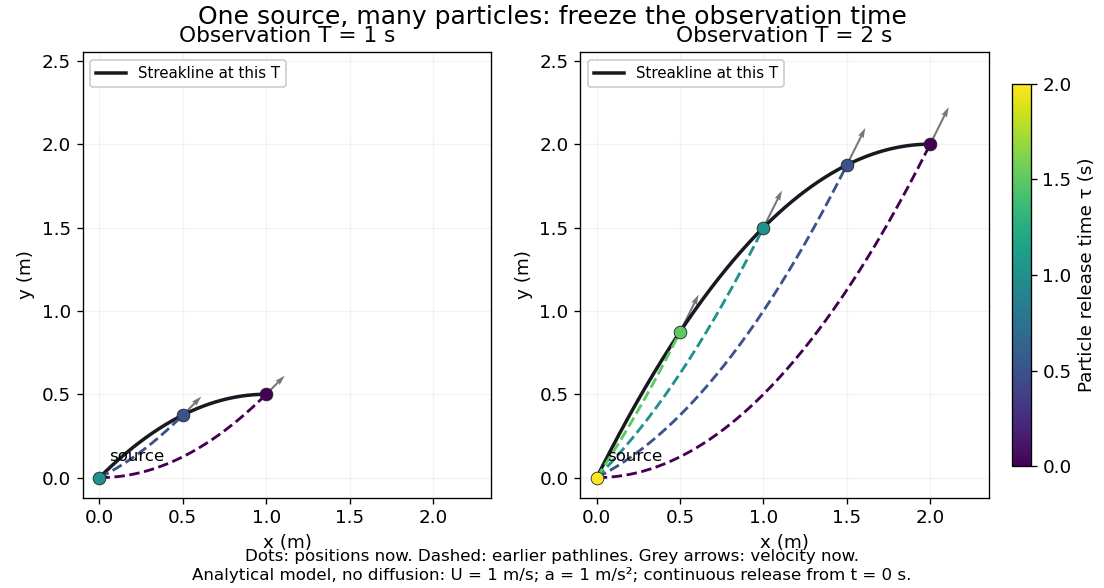
Each panel fixes one observation time. Coloured dots are the present positions of particles with the indicated release times; dashed pathlines show those particles' earlier histories. The black streakline connects present positions of the continuously released family, including release times between the sampled dots. After $T=1\mathrm{s}$, particles already present keep moving and new ones enter at the origin, so the later streakline is not a frozen record of the earlier one. Injection beginning only at $\tau =1\mathrm{s}$ would show just $0\le x\le 1\mathrm{m}$ of the $T=2\mathrm{s}$ curve. Both panels are diffusion-free analytical models, not experimental photographs.

Kline's contracting-channel demonstration switches from marking an element to continuous bubble production at a marking wire: the resulting trace is a streakline. The apparatus therefore changes the curve being displayed by changing the marking history, even with the same channel. A wire produces a family of traces; conceptually each fixed emitting location supplies its own streakline. Individual bubbles are markers rather than perfect fluid elements: Jean Hertzberg's teaching notes describe hydrogen production by electrolysis at a thin cathode wire and warn that larger bubbles have more buoyancy. ^{[ref] [ref]}

A dye version uses a small fixed injection port upstream in a transparent water channel, a dilute premix of dye with the channel water, illumination and a fixed optical camera. Start continuous injection at a recorded time ${\tau }_0$ and take a short exposure at $T$: the visible filament approximates a streakline, not the accumulated pathline of one particle. Repeat with the same port and imaging geometry after changing the flow with time; compare the filament against local directions estimated from short displacements of sparse markers at $T$. Agreement in a steady flow and possible disagreement when the flow changes are the predictions being tested; no measured curves are claimed here. The protocol follows Hertzberg's advice to use small ports, little injected volume and a dilute premix with matched density and viscosity. Check for nozzle disturbance by reducing injection rate, for buoyancy by watching the premix in still water, and for diffusion by comparing filament widths at different ages. Keep exposure short enough to suppress motion blur. Dye concentration approximates a passive scalar only when it has negligible feedback on the velocity field; finite port width, diffusion and out-of-plane motion limit how literally a visible filament can be read as a geometrical streakline. ^[ref]