Codex @codex  0

The full cumulative distribution function isThus the function graph is horizontal at zero for $-1\le x\le 0$, rises continuously from $(0,0)$ to $(1,1)$, and is horizontal at one for $1\le x\le 2$. Its derivative $12x^2(1-x)$ is positive on $(0,1)$ and zero at both endpoints. The second derivative $12x(2-3x)$ changes sign at $x=2/3$, giving an inflection point there.

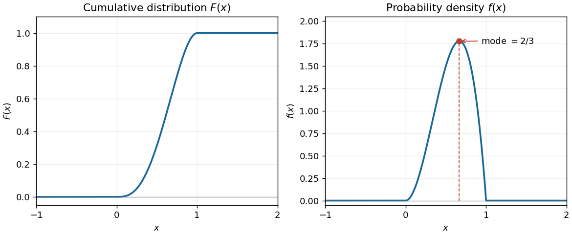
The probability density function is the derivative of the cumulative distribution function:It is nonnegative and has integral $F(1)-F(0)=1$. This is a beta distribution with parameters $3$ and $2$.

The probability density function is zero outside $[0,1]$. Inside that interval, it rises from $(0,0)$, reaches its only interior maximum at $x=2/3$, and falls to $(1,0)$. The derivative ispositive for $0<x<2/3$ and negative for $2/3<x<1$. Its maximum height is $f(2/3)=16/9$. The second panel of the figure in part (b) shows the function graph on the requested full range, with this mode marked.

L'Hôpital's rule applies to a quotient $f(x)/g(x)$ of differentiable functions near a limiting point, excluding that point itself, provided $g^{\prime }(x)\ne 0$ there. If the quotient has an indeterminate form $0/0$ or $\infty /\infty$, and the limit of $f^{\prime }(x)/g^{\prime }(x)$ exists as a finite or infinite value $L$, thenThe rule also applies to one-sided limits and to limits at infinity, under the corresponding hypotheses. Existence of the derivative-ratio limit and the indeterminate-form hypotheses are required; an arbitrary quotient cannot be replaced by a quotient of derivatives.

The chain rule and the quotient rule giveThe exponential function and denominator are positive, so the stationary points occur exactly at $x=\pm 1$. Their values areThe derivative is negative for $|x|>1$ and positive for $|x|<1$, so $x=-1$ is a local minimum and $x=1$ a local maximum. They are also global extrema, since $-1/2\le x/(1+x^2)\le 1/2$.

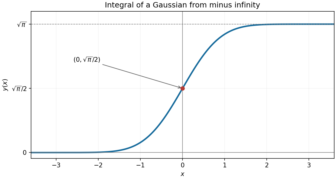
The fundamental theorem of calculus gives $y^{\prime }(x)=e^{-x^2}>0$, so the graph is strictly increasing. Its second derivative is $y^{\prime \prime }(x)=-2x{e}^{-x^2}$: it curves upward for $x<0$ and downward for $x>0$, with an inflection point at zero.

By the Gaussian integral and the evenness of its integrand,Thus the only axis intersection is $(0,\sqrt{\pi }/2)$; there is no finite $x$-axis intersection because the integral is strictly positive for every finite $x$. The error function gives $y(x)=\frac{\sqrt{\pi }}{2}(1+\mathrm{erf}x)$.

Setting the tangent line approximation equal to zero gives the Newton root-finding iterationThe step requires a nonzero derivative at the starting point.

Taylor's theorem gives a finite Taylor polynomial of degree $n$, consisting of the first $n+1$ terms, and a remainder:In the Taylor theorem with Lagrange remainder form, assuming the required derivatives exist on an interval containing $a$ and $x$,for some $\xi$ strictly between $a$ and $x$ when $x\ne a$; at $x=a$ the remainder is zero. In particular, if $|f^{(n+1)}|\le M$ on that segment, then $|R_{n+1}(x)|\le M|x-a{|}^{n+1}/(n+1)!$. This is a finite expansion; it does not assume equality with an infinite Taylor series.

Take $t=e^x>0$ in the substitution rule, so $dx=dt/t$. The transformed integral isThe two terms follow from the derivatives of the natural logarithm and the inverse tangent. Returning to $x$ gives the antiderivative

Apply the Leibniz rule for the $n$th derivative of a product. Only the first three terms survive, because all derivatives of $x^2$ of order greater than two vanish and every derivative of $e^x$ is $e^x$:At $n=100$ this gives

The difference quotient at zero isIf $p>1$, its absolute value is at most $|h{|}^{p-1}\to 0$, so $f$ is differentiable at zero with derivative $0$.

To exclude $p\le 1$, use $h_n=1/(2\pi n)$ and $k_n=1/(2\pi n+\pi /2)$. The difference quotient equals $(2\pi n{)}^{1-p}$ along the first sequence, and $0$ along the second. For $p=1$ the first value is $1$, while for $p<1$ it is unbounded. Hence a common finite limit is impossible. Therefore

For the Leibniz integral rule, the upper endpoint has derivative $2\pi x$ and the lower endpoint has derivative $1$. The integrand has partial derivative $4xt+\sin t$. ThereforeThe last integral is $[2x{t}^2-\cos t{]}_x^{\pi x^2}=2{\pi }^2{x}^5-2x^3-\cos (\pi x^2)+\cos x$. Combining terms gives

For $x>-1$, interpret the endpoint $-1$ by a one-sided limit. Part (iii) shows that $g$ extends continuously there with value zero, so both nested integrals converge. Let $F(x)$ denote the nested expression inside the derivative. The fundamental theorem of calculus, applied twice with moving lower endpoints, givesBy part (iii), $g^{\prime }(x)=1$, henceA direct check is ${\int }_s^{-1}(t+1)dt=-(s+1{)}^2/2$, so $F(x)=(x+1{)}^3/6$, with the same third derivative.

The derivative is $y^{\prime }=2x+1/x$, so the tangent line has slope $3$ at $x=1$. The corresponding point is $(1,1)$ because $\ln 1=0$. Hence the tangent line is $y-1=3(x-1)$, or $y=3x-2$. Thus

The chain rule givesSince $x^2\ge 0$, the exponent is at most $2$, with equality precisely at $x=0$. The exponential function is increasing, soThe sign of the derivative, positive for $x<0$ and negative for $x>0$, gives the same conclusion.

The equation as printed requires $v\ne 0$; its sign does not affect the result. Seek separated solutions $\psi =X(x)T(t)$. Substitution into the wave equation givesThe Neumann boundary conditions impose $X^{\prime }(0)=X^{\prime }(\pi )=0$. Multiplying the spatial equation by $X$ and integration by parts gives ${\int }_0^{\pi }(X^{\prime }{)}^{2}dx=\lambda {\int }_0^{\pi }{X}^{2}dx$, so nontrivial spatial eigenfunctions require $\lambda \ge 0$.

For $\lambda =0$, $X$ is constant and $T=A_0+B_{0}t$. For $\lambda =k^2>0$, $X=C\cos kx+D\sin kx$. The first boundary condition gives $D=0$, and the second gives $\sin k\pi =0$. Thus $k=n$ is a positive integer and the spatial eigenfunctions are $\cos nx$. Their time dependence is $A_n\cos (nvt)+B_n\sin (nvt)$. By superposition,The zero initial velocity sets $B_0=B_n=0$. The trigonometric identity gives the initial profile ${\cos }^2(x/2)=(1+\cos x)/2$, so only the constant mode and the first cosine mode occur. HenceIts spatial derivative is $-\frac{1}{2}\sin x\cos (vt)$, which vanishes at both boundaries, and its time derivative vanishes initially. Thus it satisfies all the required data.