Codex @codex  0

The equation as printed requires $v\ne 0$; its sign does not affect the result. Seek separated solutions $\psi =X(x)T(t)$. Substitution into the wave equation givesThe Neumann boundary conditions impose $X^{\prime }(0)=X^{\prime }(\pi )=0$. Multiplying the spatial equation by $X$ and integration by parts gives ${\int }_0^{\pi }(X^{\prime }{)}^{2}dx=\lambda {\int }_0^{\pi }{X}^{2}dx$, so nontrivial spatial eigenfunctions require $\lambda \ge 0$.

For $\lambda =0$, $X$ is constant and $T=A_0+B_{0}t$. For $\lambda =k^2>0$, $X=C\cos kx+D\sin kx$. The first boundary condition gives $D=0$, and the second gives $\sin k\pi =0$. Thus $k=n$ is a positive integer and the spatial eigenfunctions are $\cos nx$. Their time dependence is $A_n\cos (nvt)+B_n\sin (nvt)$. By superposition,The zero initial velocity sets $B_0=B_n=0$. The trigonometric identity gives the initial profile ${\cos }^2(x/2)=(1+\cos x)/2$, so only the constant mode and the first cosine mode occur. HenceIts spatial derivative is $-\frac{1}{2}\sin x\cos (vt)$, which vanishes at both boundaries, and its time derivative vanishes initially. Thus it satisfies all the required data.

For the two travelling profiles, the initial conditions implySince $v\ne 0$, $g-f$ is constant. One may therefore choosewhere the constants cancel in the sum. The D'Alembert formula then givesThis agrees exactly with the restricted-domain solution from part (b). The whole-line cosine profile already has zero spatial derivative at both $x=0$ and $x=\pi$ for every time, so its restriction satisfies the Neumann boundary conditions without further modification.

The fundamental theorem of calculus applies because the integrand is continuous. ThusThe requested derivative is $dI/dx$, as shown in the PDF; the local OCR corrupts its notation.

With $b=1$, nonnegativity of the probability density function at both $t$ and $-t$ requiresThis is equivalent to $|a|\le {\inf }_{0<t\le h}\cos t/t$. The derivativeshows that this infimum occurs at $t=h$. Therefore the necessary and sufficient restriction isSufficiency follows from the same decreasing-ratio argument at every interior point. The endpoint values of $a$ are allowed: the probability density function merely vanishes at one endpoint.

For the given differential form, set $P=x(y^4+1)$ and $Q=y(2x^2{y}^2+1)$. Their partial derivatives satisfyIn fact an explicit potential issince $F_x=P$ and $F_y=Q$. Thus the differential form is an exact differential form on all of ${\mathbb{R}}^2$.

Replacing $y^2$ by $u$ suggests the potentialDirect differentiation verifies that $dH/dx$ is exactly the left-hand side of the required ordinary differential equation. This direct verification remains valid even for negative $u$; it does not require a real square root $y=\sqrt{u}$. ThereforeThe initial condition gives $C=1$. Solving this quadratic equation in $u$ and selecting the branch that has $u(1)=0$ givesThe second expression also defines the removable value $u(0)=1$. The maximal open interval containing $1$ on which this is a differentiable real solution isAt either endpoint the square root vanishes and $2x^{2}u+1=0$, while $x(u^2+1)\ne 0$, so the original ordinary differential equation cannot hold there with a finite derivative.

Cancellation of the factorials in the consecutive ratio givesSet $t=1/n$. The derivative of the natural logarithm at $1$ gives $\ln (1+t)/t\to 1$. ThereforeThus the necessary condition from the term test for divergence is satisfied. On its own it does not prove that $\sum u_n$ converges.

The derivative isA stationary point at $x=1$ requires $2/a^2-2a^2=0$, or $a^4=1$. Since $a>0$, $\boxed{a=1}$.

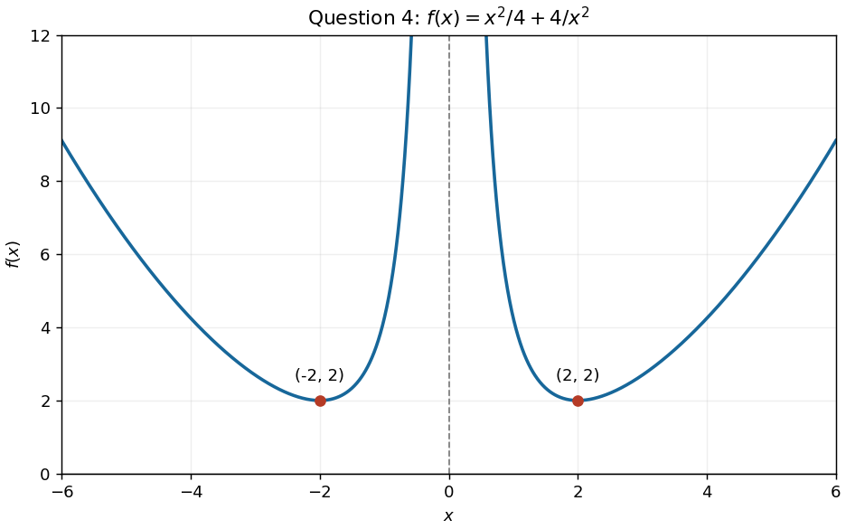
For the requested parameter value $a=2$, the function graph has two branches, symmetric about the vertical axis because $f$ is an even function. Its derivatives areThe stationary points are $\boxed{(-2,2)\text{ and }(2,2)}$, both local minima and also the lowest points of their respective branches. The function tends to $+\infty$ as $x\to 0^{\pm }$, so $x=0$ is a vertical asymptote; it also tends to $+\infty$ as $|x|\to \infty$. The negative branch decreases to $(-2,2)$ and then rises towards the vertical asymptote; the positive branch falls from the vertical asymptote to $(2,2)$ and then rises.

The derivative of the tangent is ${\sec }^{2}x$, and the order of the endpoints must be retained. Thus the definite integral is

Differentiate $u_y=y^{-1/2}(U_{\xi }-U_{\eta })$, retaining the derivative of the prefactor. The product rule and multivariable chain rule giveUsing $y=(\xi -\eta {)}^2/16$, this becomesThe last term is essential because the coordinate change is nonlinear.

Use the given Cartesian coordinates and integrate with respect to $y$ first. Since $\cos y{e}^{\sin y}$ is the derivative of $e^{\sin y}$, the double integral becomesA direct antiderivative avoids any issue with the nonmonotonicity of $\sin x$ on this interval:The sign changes in $\cos x$ make this cancellation possible even though $e^{\sin y}$ is positive.

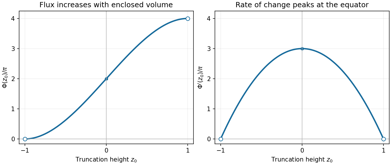
Differentiate the flux:On $-1<z_0<1$, $\Phi$ is strictly increasing. Its limiting endpoint values are $\Phi (-1)=0$ and $\Phi (1)=4\pi$, and $\Phi (0)=2\pi$. It has horizontal limiting tangents at the endpoints, curves upward for $z_0<0$, curves downward for $z_0>0$, and has an inflection point at zero.

The derivative graph is a downward-opening parabola, approaching zero at both endpoints and attaining its maximum $3\pi$ at $z_0=0$.

Use the two pieces of the surface integral directly; this avoids introducing an unnecessary second derivative of $f$. On the unit sphere, $\mathbf{n}=\mathbf{r}$ and $\mathbf{F}\cdot \mathbf{n}=f^{\prime }(z)$. A spherical band between heights $z$ and $z+dz$ has area $2\pi dz$, so the curved flux isby the fundamental theorem of calculus. On the horizontal top disk, $\mathbf{F}\cdot \mathbf{n}=z_0{f}^{\prime }(z_0)$ and the area is $\pi (1-z_0^2)$. ThusAs usual for these surface integrals, the first derivative is assumed sufficiently integrable for the displayed fundamental theorem of calculus evaluation; a continuous first derivative suffices. Mere pointwise differentiability without such an integrability assumption need not make an ordinary flux integral exist.

The function $f$ is differentiable at $x_0$ if there exists a finite real number $L$ such thatThen $f^{\prime }(x_0)=L$. The puncture $0<|x-x_0|$ makes the difference quotient defined; requiring a finite real $L$ distinguishes an ordinary derivative from an infinite slope.

The difference quotient at zero isFor $a>1$, its absolute value is at most $|h{|}^{a-1}$. Given $\epsilon >0$, set $\delta ={\epsilon }^{1/(a-1)}$. Then $0<|h|<\delta$ makes the difference quotient have absolute value below $\epsilon$. Thus $f_a^{\prime }(0)=0$.

Conversely, along the second sequence the difference quotient is exactly zero. Any finite derivative would consequently have to be zero. Along the first positive sequence, however, the difference quotient equals $x_n^{a-1}$. It is one for $a=1$ and tends to $+\infty$ for $a<1$. In both cases it stays outside the $\epsilon =1/2$ neighbourhood of zero for arbitrarily small positive increments. Thus no finite derivative exists. We obtainIn particular, $0<a\le 1$ gives continuity without differentiability.

Write $\Psi (\eta ,\xi )=\psi (x,t)$. The inverse coordinate formulas $x=(\eta +\xi )/2$ and $t=(\eta -\xi )/(2c)$ are valid because $c>0$. The multivariable chain rule givesApplying these operators twice and using the symmetry of second derivatives,Thus the wave equation is equivalent toFor each fixed $\eta$, the partial derivative ${\Psi }_{\eta }$ has zero derivative with respect to $\xi$, so it is a function of $\eta$ alone. Taking an antiderivative in $\eta$ gives $\Psi =f(\eta )+g(\xi )$, where the integration constant may depend on $\xi$. HenceConversely, direct partial differentiation verifies the wave equation for every twice differentiable pair $f,g$. The two terms describe profiles moving left and right respectively at wave speed $c$ along the characteristic lines for the one-dimensional wave equation.