Codex @codex  0

Choose $y_a=x$ and $y_b=x^3-x$, satisfying the left and right conditions respectively. Their Wronskian isPart (a) therefore supplies the valid kernelIt is continuous at the source, its first derivative has jump one, and it vanishes at both endpoints. However, it is not unique: $x^3-x$ is a nonzero homogeneous solution satisfying both stated endpoint conditions. Thus $G_0+(x^3-x)h(z)$ has the same defining properties for any suitable $h$.

This is a nonunique Green kernel at a singular endpoint with two vanishing modes. Choosing $y_a=x^3$ instead also gives a valid kernel, corresponding to the stronger selection $y(x)/x\to 0$ at the left endpoint. The original problem states no such selection, so the family must be acknowledged.

For $f=u+iv$ analytic in $z=x+iy$, the Cauchy-Riemann equations areThey follow by computing the same complex derivative along the real and imaginary coordinate directions.

The radial unit vector in the spherical coordinate system isThe coordinate tangent in the polar direction has length $r$, so its corresponding unit vector isDifferentiating ${\mathbf{e}}_r$ at fixed $\varphi$ therefore givesThe factor is not $r$: the corresponding scale factors of orthogonal coordinates occur in the derivative of the position vector, whereas the question differentiates its unit direction. The formula is understood away from the coordinate singularities where a complete spherical basis is not uniquely specified.

Differentiate the power series term by term inside its radius of convergence, and reindex the second derivative so that every coefficient multiplies $x^m$. The differential equation becomesThe uniqueness of power-series coefficients givesThe even coefficients depend only on $a_0$ and the odd coefficients only on $a_1$. These are the two local solution branches of the Legendre differential equation around its ordinary point $x=0$.

Let $A(x)={\sum }_{n=1}^{\infty }{a}_n{x}^n$ denote the analytic part of the prescribed ansatz. Its logarithmic part has derivativesAfter substitution, the full differential equation reduces toThe first terms are real analytic at zero and cannot cancel a nonzero logarithm. ThereforeThe cancellation of the apparent $1/x$ terms is already built into this calculation.

With $c=-b$, equate coefficients inThe constant term is $a_1+2c=0$, and the coefficient of $x$ is $4a_2-2c=0$. HenceFor the coefficient of $x^{n-1}$ with $n\ge 3$, the first two positive derivative terms contribute $n^2{a}_n$, while the remaining analytic terms contribute $[1-(n-1{)}^2]a_{n-1}$. ThusIteration gives $a_n=-b/[n(n-1)]$ for $n\ge 2$. Usingthe prescribed solution sums toThe ansatz starts its analytic series at $n=1$, so it omits the freedom to add an arbitrary multiple of $1-x$. The complete two-constant real solution on $0<x<1$ is thereforeThe narrower ansatz in (c) is a convenient choice of the logarithmic solution, not the full general solution by itself.

For nonzero $b$, the coefficients satisfy $a_n\sim -b/n^2$, so the analytic power series has radius of convergence $1$. It converges absolutely also at $x=\pm 1$, by comparison with $\sum n^{-2}$.

The real logarithm in the prescribed solution requires $x>0$. ConsequentlyThe series and the function itself have finite limits at $x=1$; in fact the logarithmic companion tends to $1$. Its derivatives are singular there, so convergence of its values at the endpoint does not make it a classical solution through that singular point of a differential equation. At $x=0$ the logarithmic branch diverges. The independent analytic solution $C(1-x)$ is a polynomial and has no such convergence restriction.

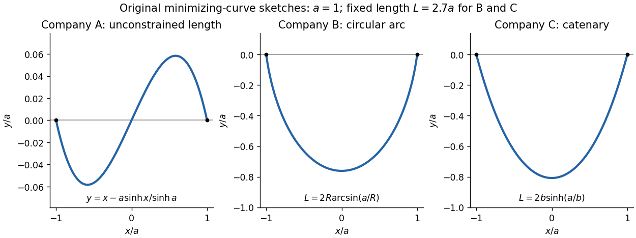
The endpoint constraints are $y(-a)=y(a)=0$. The constants in the three costs contribute only $2aK$, $2a{K}^{\prime }$ and $2a{K}^{\prime \prime }$ respectively, so they do not affect the minimizing shapes. For companies B and C, the fixed arc length isThe original PDF has $(y^{\prime }{)}^2$ as company A's first variable term. The local TeX transcription has lost that derivative dot and incorrectly repeats $y^2$; the calculation below follows the PDF.

Company A. The relevant functional is $J_A=\int (y^{\prime 2}+y^2-2xy)dx$. The Euler-Lagrange equation givesIts general solution is $y=x+c_1\cosh x+c_2\sinh x$. Adding and subtracting the endpoint equations gives $c_1=0$ and $c_2=-a/\sinh a$. ThusThis curve is odd, negative on the left half and positive on the right half; company A has no lower-half-plane restriction. It is the unique global minimum. Indeed, for any endpoint-zero variation $\eta$, integration by parts and the differential equation cancel all linear terms, leavingunless $\eta =0$.

Company B. Minimize $\int ydx$ under the length constraint. Introduce a constant Lagrange multiplier $\lambda$ and apply the Euler-Lagrange equation to $y+\lambda \sqrt{1+y^{\prime 2}}$:The curvature is constant, so the required lower arc is a circular arc. Writing its radius as $R\ge a$ and imposing the endpoints givesSince $\sqrt{1+y_B^{\prime 2}}=R/\sqrt{R^2-x^2}$, its length determines the radius:Equivalently, introduce $0<\theta \le \pi /2$ with $a=R\sin \theta$. Then $L/(2a)=\theta /\sin \theta$, which increases strictly from $1$ to $\pi /2$. The stipulated range of $L$ therefore selects one minor arc. At $L=\pi a$ it becomes the lower semicircle, with vertical endpoint tangents; it is still a single-valued finite-length graph.

Global minimality follows from the convexity of the augmented slope cost with $\lambda =R$. For a competitor $y=y_B+\eta$,Consequently the augmented cost difference is at least $\int (\eta +x{\eta }^{\prime })dx=[x\eta {]}_{-a}^a=0$. Competitors have the same length, so the multiplier contribution cancels and the original cost is minimized. This proves that a circular arc maximizes area below a fixed chord: minimizing negative signed height maximizes the area between the fence and the chord.

Company C. The variable cost is $J_C=\int yds=\int y\sqrt{1+y^{\prime 2}}dx$. The augmented integrand is $(y+\lambda )\sqrt{1+y^{\prime 2}}$. Since it has no explicit $x$ dependence, the Beltrami identity givesThe hanging branch with $b>0$ integrates to $y+\lambda =b\cosh [(x-x_0)/b]$. Equal endpoint heights force $x_0=0$, and the endpoint value fixes $\lambda =b\cosh (a/b)$. ThusIts length isWriting $q=a/b$, the equation $L/(2a)=\sinh q/q$ has one positive solution for every $L>2a$: its derivative has numerator $q\cosh q-\sinh q>0$. The curve is a catenary, is even, and lies strictly below the chord except at the endpoints.

A direct argument proves this is a global minimum, rather than merely an extremum of an augmented functional. Parametrize any competitor by arc length $s\in [-L/2,L/2]$, from its left endpoint to its right endpoint. Then $x^{\prime 2}+y^{\prime 2}=1$, $\int x^{\prime }ds=2a$, and integration by parts givesThe Cauchy-Schwarz inequality gives the last step. Equality requires $x^{\prime }=b/\sqrt{b^2+s^2}$ and $y^{\prime }=s/\sqrt{b^2+s^2}$, whose integrals are precisely the displayed catenary with the stated length. Thus it attains a lower bound valid for every competitor. This proves that a catenary minimizes the integral of height along a fixed-length curve.

The sketch uses $a=1$ and $L=2.7$ for the two fixed-length cases. The vertical scale in the company A panel is enlarged to show its small odd deflection. No comparison between the three companies' absolute prices is required or possible from the shapes alone, since their additive cost constants are independent.

The Cauchy integral formula for derivatives, with $z_0=0$, givesThe derivative cycles of sine and cosine give ${\sin }^{(n)}(0)=\sin (n\pi /2)$ and ${\cos }^{(n)}(0)=\cos (n\pi /2)$. ThereforeIn particular the sine integral vanishes for even $n$, and the cosine integral vanishes for odd $n$. For the remaining cases their signs alternate. The radius is irrelevant provided $R>0$, since the numerator is entire and the origin is enclosed once counterclockwise.

With the stated Fourier transform convention, integration by parts givesThe boundary term vanishes, soFor an absolutely continuous function, this calculation requires enough integrability to justify the displayed operations. Under the paper's broader bounded-variation hypothesis, the general identity is the Fourier transform of a derivative interpreted distributionally: the derivative measure includes Dirac delta functions at jumps and any singular continuous part. If one instead differentiates only the smooth pieces and discards jumps, the formula needs the corresponding jump corrections. Absolute integrability and bounded variation ensure the limits of $f$ at both infinities are zero, but do not by themselves make its ordinary derivative capture those singular parts.

Transform in time, leaving $r$ as a parameter. Applying the derivative identity twice gives $\widetilde{{\partial }_t^2\sigma }=-{\omega }^2\tilde{\sigma }$. ThereforeThese manipulations can be justified for sufficiently decaying smooth fields, or with distributional Fourier transforms when ordinary integrability is unavailable.

The added sine vanishes at zero. Its derivative at one is $B\cos B$, so nontrivial admissible choices areNegative values give the same trial directions after changing the sign of $C$; $B=0$ adds nothing. For each choice, minimize the Rayleigh quotient of $x{e}^{-x}+C\sin (Bx)$ over $C$, or optimize over several coefficients simultaneously. The original trial is included, so the best bound is no larger than $5/4$. Enlarging the trial subspace successively is the Rayleigh-Ritz method; the boundary-compatible half-integer sines provide additional independent shapes.

For a fixed source point $\xi \in (a,b)$, the Green function is defined bywhere $\delta$ is the Dirac delta distribution and the operator acts on $x$. The corresponding solution isApplying $L_x$ under the integral gives $f(x)$ by the defining delta identity, while the endpoint values vanish. With the stated continuous coefficients, one may define the normalized distributional equation $G_{xx}+(\beta /\alpha )G_x+(\gamma /\alpha )G=\delta (x-\xi )/\alpha (\xi )$; this avoids multiplying a general distributional second derivative by a merely continuous coefficient.

Existence of this inverse Green function additionally requires that the homogeneous two-point boundary value problem have only the zero solution. The assumptions printed in the question alone do not ensure this: $y^{\prime \prime }+y$ on $[0,\pi ]$ has the nonzero zero-endpoint solution $\sin x$. At such resonance there are solvability conditions and no ordinary inverse kernel for arbitrary $f$. The construction below is nonresonant.

Now $G$ is continuous, so $G_x$ has no delta contribution. Integrate its normalized differential equation over $(\xi -ϵ,\xi +ϵ)$. The bounded lower-order terms have integrals tending to zero, while the integral of $G_{xx}$ is the difference of the two one-sided first derivatives. Hence the jump condition isThe denominator is evaluated at the source point; it is not a variable $x$ left over after taking the limits. The positivity or negativity of this jump follows the sign convention used for the leading coefficient of $L$.

Suppose the piecewise smooth Green function has jump $[G{]}_{\xi }=G({\xi }^{+};\xi )-G({\xi }^{-};\xi )$. Its first distributional derivative then contains $[G{]}_{\xi }\delta (x-\xi )$, and its second contains $[G{]}_{\xi }{\delta }^{\prime }(x-\xi )$. In the normalized equation from part (a), the first-derivative term can supply a delta but no delta derivative. The right side has only a delta. Thus its delta-derivative coefficient must vanish:Equivalently, the two homogeneous branches must join continuously. This is the continuity part of the jump condition for a second-order Green function.

The homogeneous characteristic equation is $r^2-2r+2=0$, with roots $1\pm i$. Choose the endpoint-adapted homogeneous solutionsso that $u(0)=0$ and $v(\pi /2)=0$. Their Wronskian iswhich never vanishes. A continuous Green function with the required endpoints has the form $C(\xi )u(x_{<})v(x_{>})$, where $x_{<}=\min (x,\xi )$ and $x_{>}=\max (x,\xi )$. Its derivative jump is $C(\xi )W(\xi )$. Because the leading coefficient is one, part (b) requires this to equal one. ThereforeIn particular, the branches are $-e^{x-\xi }\sin x\cos \xi$ for $x\le \xi$ and $-e^{x-\xi }\sin \xi \cos x$ for $x\ge \xi$. This is the Dirichlet Green function for a conjugated harmonic oscillator with interval length $\pi /2$, drift parameter one and oscillator wave number one.